
BlurXTerminator - A Breakthrough in Deconvolution?
Jan 17, 2023

1-26-23 Update Notice:
Russell Croman has recently had an interview where he talked about BlurXTerminator, and based on the new information presented there, I have updated portions of this article. Those updates will be colored light blue for easy identification. In addition, Russell has published a video of a 2022 AIC Presentation describing the technology approach he used. A link for that video is included in the section talking about the technology.
Table of Contents Show (Click on lines to navigate)
Companion Video
I0-21-23: I just posed a companion video to this article on my YouTube Channel, which can be shown below. I have been trying to do a reasonably short video with each article to introduce the topic and discuss some aspects of the article. I failed in this case, as the video is almost an hour long! I will endeavor to create shorter videos for articles in the future!
To help you navigate through this video, I added a timestamp roadmap in the description of the video, showing what is covered and where it can be found. Hope that helps!
Some Background
I began my journey into Astrophotography just over three years ago now.
In making this journey, there was so much that had to be learned. Configuring a telescope system, setting up your equipment properly, learning how to collect data, and finally - learning how to calibrate and process the data you have collected.
Of all of the things I had to learn, I found learning to effectively use Deconvolution to be one of the hardest skills for me to acquire!
Understanding what PSF is and how to create a PSF file suitable for use in deconvolution
Learning how to make good Object Masks to protect low-signal areas
Understanding how to avoid local ringing on bright stars by creating and using a Local Deringing Support image
Learning how to test for parameter combinations to get the best results and avoid artifacts
Learning to use the Regularization parameters so that the Object Mask was no longer needed
Learning to use the EZ-Decon tool
Learning the right workflow to use deconvolution to advantage
But learn it, I did. Slowly, until I reached the point where I could consistently get good results.
I had such a hard time with it that I decided to create a tutorial for my website so I could share what I had learned.
When it was done, It was so long and detailed that I broke it into a 7-part series - and then I did two follow-up posts discussing the use of EZ-Decon and The use of Regularization. Whew!

Part 2 - An Overview of PFS and Deconvolution (You are here)
Follow-up: Using Richardson-Lucy Wavelet Regularization Parameters in Pixinsight Deconvolution
There is a lot to deconvolution! It is a very powerful tool, but it is also a tool that has many parameters that must be intelligently set otherwise, it will do more harm than good. So you must understand it and its failure modes and develop the skills for achieving good results whilst avoiding harm.

BlurXTerminator Is Released!
Then I saw that Russell Croman Astrophotography had released BlurXTterminator. I was super excited upon learning of this!
By why? I didn’t even know what the tool did yet!
I was excited because I have been a customer of Russell’s for a while now and have been extremely impressed with his previous software offerings. Russell is using smart Machine Learning technologies trained on astrophotographic data to solve tough problems in astrophotography:
NoiseXterminator - this tool revolutionized how I do Noise Reduction. Instead of using a handful of difficult-to-use tools in Pixinsight, I now use NoiseXterinator exclusively to do nose reduction for linear and nonlinear data. Simple and intuitive to use, I love this tool!
StarXterminator - this tool does star removal so well that I changed my workflows to go starless for the first time. I had tried to do this with Starnet and Starnet2, but I always ran into artifacting issues. Not so with StarXTerminator!
These tools proved to me that AI Network Technology - when trained with Astrophotographic data - could do outstanding work. I also saw significant improvements in the tools over time, as the training was improved and the resulting networks were released to users.
BlurXTerminator claimed to use this same technology to do deconvolution!
My First Impression of BlurXTerminator
So I downloaded the trial version and tried it out quickly. With my very first test, I was blown away!
Simple to use
Control of how it operated on stars vs. non-stars!
Control of how it operated on star cores vs. halos!
The ability to deal use of differential PSFs across the field (which PI Decon cannot do)
The ability to deal with and correct distorted and truncated PSFs! (again, something that PI Decon cannot do)
The more I played with it, the more impressed I was. A friend of mine, Dan Kuchta, tried it out and said, "Shut up and Take my Money!" That about sums it up.
I told my local colleagues that I needed to add another chapter to my now 9-part series on deconvolution.
Here is the total text I proposed for the new article:
"Remember my 9-part deconvoution series ? Well just forget all of that crap and buy BlurXTerminator. The End"
I shared that I was working on a new post and video for my YouTube channel - based on this one line of text, and I got the following response from Loran Hughes:
Does Youtube accept videos under 10 seconds? 🤣🤣
— Loran Hughes 🪐 Westwood Astro 🔭 (@LoranHughes) January 13, 2023
I replied that he greatly underestimated my ability to talk for a very long time about very little!
Well, here I am writing the new post - I must say it will be a bit more involved than that single line of text. It will be longer because I would like to share my experience with it, provide a level overview of the Machine Learning technology that it is based on, and address some recent pushback I have been seeing around this tool.
Pushback on BlurXTerminator?
There has been a strong reaction to the release of BlurXTerminator. Strong good, and surprisingly to me, some strong bad reactions.
I fully understand the good reactions because, in my mind, it is richly deserved. The tool delivers a breakthrough capability.
But the bad reactions? These seem to fall into three camps from what I have seen.
The Sour Grapes Camp
There is no doubt that it is hard to learn to use deconvolution effectively.
If you have reached a point where you can use Decon well - you’ve had to climb a mountain to get there. You are part of the more elite group of Astrophotographers. You have earned your stripes and are proud of it.
Then BlurXTerminato comes along, and suddenly any Tom, Dick, or Harry can use decon as well or better than you can! The nerve of it all! How dare they do this without having worked hard to earn the right!?
This group of people seems to feel that their elite status is being challenged. So I guess that means that BlurXTerminator must be a bad thing…
The Conspiracy Theory Camp
Most of what I have seen in this category seems to come from people that clearly do not understand Machine Learning, Neural Networks, and related AI technologies. They don’t know what it is, what does, or how it does it. It seems awfully good - perhaps too good!
Since they don’t understand it, they decide what to believe about how it must work. This clearly seems to involve doing unethical things which are wrong and should not be embraced:
It replaces your pixels with Hubble pixels or someone else’s pixels! (It does NOT!)
The AI was trained on Hubble and JWST images, and who knows what the AI is really doing - but it can’t be good and is really a form of cheating! (Cheating? - Hogwash!)
The “Issue of Trust” Camp
Neural Networks are complex beasts, and understanding how they work once trained is not something that can be easily done. Because of this, there is another camp that is just not sure that they trust the operation of the tool. Perhaps it makes your image look good - but how do you know that the result is correct and “right.” How do you know that what it does in all circumstances is what should have been done? These folks have some legitimate questions, and they will likely require more scrutiny of BlurXTerminator before they are ready to adopt it.
I have no problem with this kind of pushback.
Any sophisticated algorithm that transforms an image in some way - be it for noise reduction, star removal, or deconvolution - attempts to solve a problem, and it will do so with some kind of error rate. It is up to the user to determine if the tool produces a result that is acceptable and compatible with their artistic vision. This is true whether the method used by the algorithm is a linear model, a statistical model, or a network model.
The biggest advantage of digital imaging and image processing is that you can change any aspect of an image.
The biggest disadvantage of digital imaging and image processing is that you can change any aspect of an image.
It's a two-edged sword.
In my mind, the concerns that are voiced in this camp are no different than concerns placed for any new tool or capability. How do you ultimately decide if it is right for you? You try it - see what it does for your image- and you decide if this is something that you want to add to your toolbag.
Thoughtful Honest Concerns vs. Making Stuff Up
If you don’t like a tool for how it works or the results it produces - that’s fine - nothing wrong with that. Your opinion on these aspects matters.
If you don’t like it for philosophical reasons - that’s fine too. I have some self-imposed rules about what I think my Astrophotography should and should not involve - but I don’t fault others for not adhering to my views.
If you are just not sure a tool is right for you - then by all means, state your opinion and make your own call.
If you have examples of performance that raises questions - by all means, share those examples. This would be a help to the community.
I have no problem with any of that.
But don’t misrepresent what a tool does or how it works. Don’t make stuff up and use that as a reason to cast shade on it. That’s just wrong on multiple levels. I have seen comments like this in several forums, and it drives me nuts. People are making claims about what it must be doing - and these claims have no basis in fact or reality.
My Experience With Neural Network Technology
I have a basic understanding of Neural Networks and related technologies.
Most of my career was spent doing R&D at Kodak, and much of that was back in the days when film was King (yeah - I know - this sure dates me!)
In the late 90s, I spent some time researching the use of Neural Networks for imaging applications. I wrote software that allowed Neural Networks to be trained and used. I created data sets for training. In those days, when computing power was a fraction of what it is today - we bought special multiple CPU networked computers that would speed up training.
At that time, we were dealing primarily with MLPs - Multi-Layered Perceptrons. Since those days, the technology of deep learning has moved on to better and more sophisticated concepts. Convolutional Neural Networks and advanced network architectures shepherded in a new era of Machine Learning solutions. Computing power has also enabled larger and faster networks.
To be clear, I am NOT an expert in Machine Learning. But I know enough about this domain to be dangerous - and talk about it a bit.
I don’t know Russell Croman, and I have never talked to him. I don’t know exactly how he has created his software solutions - but I have a pretty good idea - enough to know that some of the pushback against it is utter hogwash.
What We Will Cover
So with that high-level overview in mind, let’s do a somewhat deeper dive. We will cover the following:
What BlurXTerminator is and how it works
Using BlurXTerminator
Comparing BlurXTerminator to Traditional Pixinsight Deconvolution
Workflow Considerations
An Overview of Neural Network Technolgy
My First Exposure to Neural Networks
Convolutional Neural Networks and Advanced Network Architectures
What RC Astro is likely to be doing with BlurXTerminator
Revisiting the Concerns Raised Around BlurXTerminator.
Let’s get started!
So what is BlurXTerminator?
For the remainder of this article, I will refer to BlurXTerminator as BXT.
BXT is an AI Tool based on Machine Learning - and what I believe is based on a Convolutional Neural Network.
There are other AI-based image enhancement tools out there - some of the first were the series of tools from Topaz Labs, which did noise reduction and sharpening on images. Early on, I bought licenses for these tools and tried to apply them to my Astrophotography - with some limited success.
We will go into some detail on Neural Network technology but let me first share that these work by being trained. Training consists of exposing the network to data sets that define the problem space. The data set you use has a huge impact on the performance of the network.
Topaz tools were trained on standard pictorial images that typical people would take.
As we all know, Astrophotographers are NOT typical people, and our Astrophotos look quite different! As a result, the Topaz tools don't always do the best job on Astro Images.
RC Astro, however, has built a series of tools that have been exclusively trained with Astro image data, and their performance shows it!
In the case of BXT, it has been trained to do deconvolution.
It samples a region of the image and assesses the stars in that region, developing a localized PSF. It then corrects the PSF and does deconvolution on that data.
RC Astro’s StarXTerminator tool demonstrates that AI technology can be trained to detect stars and remove them effectively. Clearly, some of this experience was leveraged for BXT. BXT provides an easy-to-use set of controls that allow you to control the sharpening of Stars - both the core and the halos, as well as non-stars.
Using BXT
Unlike too many tools in Pixinsight, BXT comes with excellent documentation, and there is a lot to be learned here.
As you might expect of a deconvolution tool, BXT is designed to be used in the linear domain very early in the processing chain. The only operations I might consider doing on the image prior to the application of BXT are:
Dynamic Cropping to eliminate bad data from ragged edges of the image
DBE to remove any gradients.
For RGB images, I would also do PCC or SPCC color correction.
I view these operations as remedial calibrations, and I would not expect them to distort the linear nature of the data set.
I have seen reports of people using BXT with nonlinear data and even applying BXT very late in the processing effort - some are claiming they are getting good sharpening results this way. Perhaps this is true - but in those cases, you are using it as some kind of a sharpening tool rather than doing a true deconvolution image restoration. In fact, when used this way, people seem to be trying to sharpen large-scale features of the image - where deconvolution is all about fine-scale restoration.
The network is trained on linear data to do fine-scale data restoration - so I would expect the best results when it is used the same way it was trained.
Unlike traditional deconvolution, BXT does not require you to do any preparation before running.
When you are ready for the deconvolution step, just run BXT, and you will see its control panel:

The Control Panel for BlurXTerminator with default values..
The first thing to note is that there are significantly fewer controls than in regular deconvolution. Controls are grouped into Stellar Adjustments, Nonstellar Adjustments, and Processing Options.
But let’s try using BXT with just the default setting. Yes - I know - running deconvolution without tweaking sounds crazy - right? But let’s give it a go.
For this example, I am using my narrowband SHO image of Metlotte 15 - The Heart of the Heart. (You can see that imaging project HERE).
I picked this image because when I first processed it, I had difficulty getting substantial improvements from decon. I did get some benefits, but I never seemed to find the sweet spot to give me great results.
The comparison below shows my starting Synthetic Luminance Image, the results I obtained from traditional deconvolution, followed by the results from BXT (run with the default settings).
Before Decon, After Decon, After BXT with Default Settings
As you review the images, you can see that I did make some improvements with traditional deconvolution. The stars are reduced, and the nebula has gained in detail and sharpness.
Then we see BXT.
The stars are dramatically reduced, and the nebula is even sharper.
Keep in mind that I probably spent almost an hour playing around with traditional deconvolution to get this result.
I spend NO time getting the BXT result! (This is not completely true - BXT took 5 minutes to run on my image.)
If the BXT results were the same as what I got with traditional BXT, but it saved me an hour of work, BXT would be worth it to me. But it gave me superior results!
This is very impressive, and I was instantly impressed!
Exploring the Controls
BXT does not have many controls, but let’s explore the controls that it does have.
Select AI Button: This button allows you to select which weight map will be used by the tool. The weight map defines the functionality of the network, and you can expect RC Astro to be updating this over time and improving the results. This has been my experience with NoiseXTerminator and StarXTerminator, and I fully expect updates here that will continue to improve the performance of BXT. I am currently using the V2 map, which has already been distributed.
Next, we have the Shapen Stars section with two slider controls:
Sharpen Stars: This slider runs from 0.0 to 0.5 and sharpens the cores of the stars. The default value is 0.25. Higher values result in smaller and sharper stars. At the maximum values, stars can be reduced in size by half. It is possible to be too aggressive here - which can result in dark rings for some images. If you see that - you have gone too far, and it is time to back off.
Adjust Star Halos: This slider controls how halos are handled. I love the ability to control the look of stars allowing me to adjust the core of the star vs. the halo of the star! This slider has a range of -0.5 to +0.5. The default value is 0.0. Higher values result in larger and brighter halos. You can dial in the look you want for a star with this control. Since a lot of the star color is found in the halo (as the center is often clipped or desaturated), this can change your perception of the stars in your image.
Now we move to the Nonstellar Adjustments section.
Automatic PSF: Selecting automatic PSF will determine the local PSF from stars in that region. One of the reasons that this is included is to make BlurXTerminator easier to use out of the box. This PSF will then be used for nonstellar correction and sharpening. If there are no stars or insufficient stars, an estimate will be made from the nonstellar areas of the image. This does not appear as robust and may not give the best or the most consistent result across the image. If you have good sample stars in the region, this should work well, and as a bonus, will apply corrections for aberrations and guiding errors.
In manual mode, the PSF that will be used is constructed from the WFHM diameter from the slider. Since it is computed rather than sensed - it does not know about aberrations or other issues and cannot correct them. It also means that no corrections are made for PSFs that might be different between the color layers.
The documentation indicates that 512x512 pixel tiles are processed, and the PSF for each tile is uniquely determined. If you end up with a lot of tiles that have few stars, then going manual may give you better results. This would most likely be the case when using a long focal-length instrument.
PSF Diameter (Pixels): In manual mode, you can specify the PSF diameter in terms of FWHM for deconvolution. Ideally, you would determine this value by looking at the sizes of stars in your current image and setting the value accordingly. Frankly - it would be nice if the tool reported some statistics from the image stars to guide you in this - but it does not. The scale goes up to 8 pixels, with the idea that stars larger than this are oversampled. My sense is that this is one of those parameters where you do need to experiment a bit to get better results. I tend to keep things on automatic, which works well for my scopes.
Russel suggests using the DynamicPSF tool to select a few non-saturated stars from the image. You can tell they are non-saturated if you can’t see the star when STF is disabled. Once you have chosen a few - hit the statistics button and see what the FWHMx and FWHMy numbers are - use these numbers in the slider, and you can get a much better result in some cases.
Oversharpening can occur if the PSF diameter used is too large. There are areas of smooth nebulosity, and if you oversharpen, you can lose that.
Sharpen Nonstellar: This sharpens nonstellar features when in manual mode. The range goes from 0.0 to 1.0, with a default value of 0.9. At the top of the scale, BXT attempts to reduce the size of a feature by the fraction specified - down to a point source. Of course, the actual sharpening is limited by the information contained in the region.
Finally, we have the Options section. These flags change the way the tool is run.
Correct Only: BXT will attempt to circularize stars that are distorted due to aberrations and guiding errors without doing deconvolution. Technically, this is transforming from a noncircular PSF to a circular PSF without doing any sharpening This will round stars out, and if there are color aberrations seen (the PSF for one color layer being different from another color layer), it will fix that as well. This is the same as using Automatic PSF and setting all other parameters to zero. Better results can sometimes be had by correcting the stars first and then doing a full restoration run.
Correct First: This is equivalent to checking Correct FIrst and then doing a full BXT run. This basically does a pass using Auto-PSF, which will correct non-round shapes and color aberrations for both stellar and nonstellar features - but apply no sharpening. Then a subsequent run is done where sharpening occurs - and for nonstellar features, this could be in manual PSF mode. This allows you to get the benefit of auto-PSF while allowing for greater sharpening PSF manual PSF for nonstellar features in some circumstances.
Nonstellar Then Stellar: This performs Nonstellar sharpening followed by Stellar sharpening. According to Russell:
This can be useful for some images, for example, galaxies with faint, barely-resolved stars embedded in other structures, such as HII regions. Stellar sharpening may not recognize these as stars at first, but if nonstellar sharpening is performed prior to stellar sharpening, these stars become resolved in the first step and then sharpened in the second step.
Luminance Only: This applies deconvolution to the Luminance channel only and disables cross-channel correction for things like Chromatic Aberrations. This mode will do a channel extraction using HSI, extract the intensity layer, apply deconvolution and then rebuild the color image. This option is meaningless if the image in question is a luminance image. Should you ever see anything strange going on colorwise, you can always use this option to disable color corrections being made.
I have found that, for the most part, these controls are intuitive and simple to use. The default values tend to do a good job, but I think most astrophotographers would be motivated to explore various setting options. The one downside here is that BXT takes time to run. So I would highly recommend creating previews on strategic portions of the image and doing parameter tests using that smaller data set when experimenting with other settings.
Let’s explore what some of these sliders do. We will start with the Sharpen Stars Slider:


Sharpen Stars slider values: 0.1, 0.2, 0.25 (default), 0.3, 0.4, 0.5
You can clearly see the stars being reduced as you move up the scale.
Now, let’s look at the Adjust Star Halos slider:


Star Halo slider values: -0.5, -0.25, 0.0 (default), 0.25, 0.5
Again, the slider seems intuitive to use and provides good control of the halos around the stars.
Let’s explore BXT’s ability to do star correction and cross-channel optimization.
Star Correction
BXT, unlike traditional Deconvolution, works with differential PSFs across the frame (based upon 512x512 tiles) and can correct (or, more precisely, circularize) stars distorted by small guiding errors, optical aberrations, and coma. Let’s explore that a bit.
My image of Melotte 15 was shot on a William Optics 132mm FLT Scope. I do not have a flattener on this scope, so I can see some optical aberrations in the extreme corners of my images. Did BXT fix these? Let’s look:
Right Bottom Corner - Before BXT Correction

Top Left Corner - Before BXT Correction

Right Bottom Corner - After BXT Correction
Top Left Corner - After BXT Correction
The correction seen in the Bottom Right Corner Image is clear - it did a really nice job of rounding out the stars. The correction for the Top Left Corner image is noticeable but not as complete. So clearly, some improvements are happening! Hopefully, over time this will improve even more!
Cross-Channel Corrections
BXT is optimized for cross-channel deconvolution. This suggests that BXT will do a good job dealing with the color aberrations of stars.
When I first started using deconvolution, I ran it on each color channel. This caused a problem since the amount of correction on each channel could be different, and when the color channels were combined, my stars ended up with color rings. Today, I apply deconvolution exclusively to Luminece images and then fold those effects into the color image using the LRGBCombination process.
It sounds like BXT can handle color images well - so let’s test that. Below is the initial color combination of the SHO image in linear space.
The SHO Linear image before BXT (click to enlarge)
SHO before BXT - Zoomed in (click to enlarge)
The SHO Linear image after BXT (click to enlarge)
SHO After BXT - Zoomed in (click to enlarge)
The color SHO image is what we normally see when first combing images: a strong green color balance and funky-looking magenta stars. But after running BXT, the stars are much smaller, and almost all hints of the magenta color have been removed! This is an impressive result and suggests that there would be a real advantage to running BXT on color images. This is enough of an effect to have me reconsider what my workflow should be for narrowband images!
Another Test
I wanted to get a feel for how BXT handles two other issues: undersampled data and overlapping stars.
In my experience, deconvolution does well when you have well-sampled data. If your data is undersampled, the stars - especially the fainter ones - can begin to get a little blocky in appearance. I have not always
gotten good results for undersampled data, as the stars become sharper blocks. This doe not really help.
Sometimes when stars are very close together, the airy disks can overlap. I wanted to see how this was handled by BXT as well.
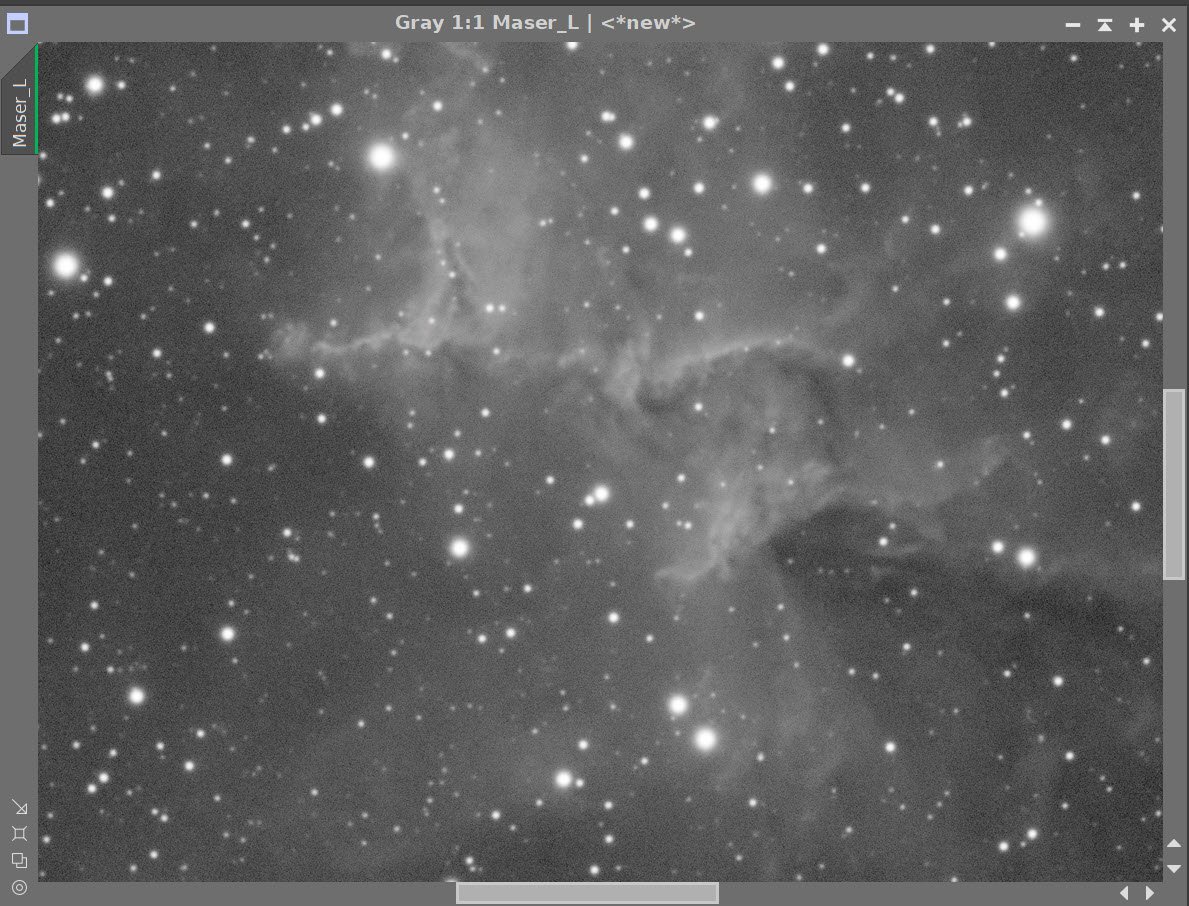
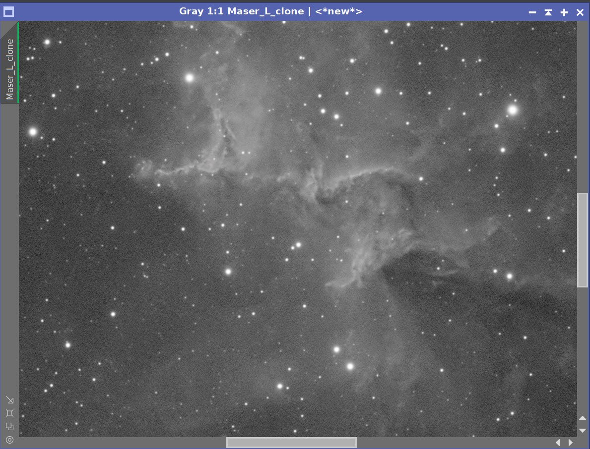
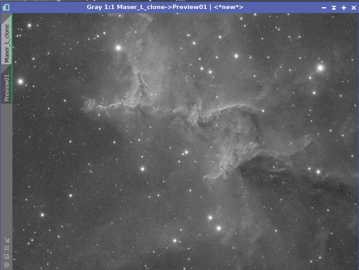
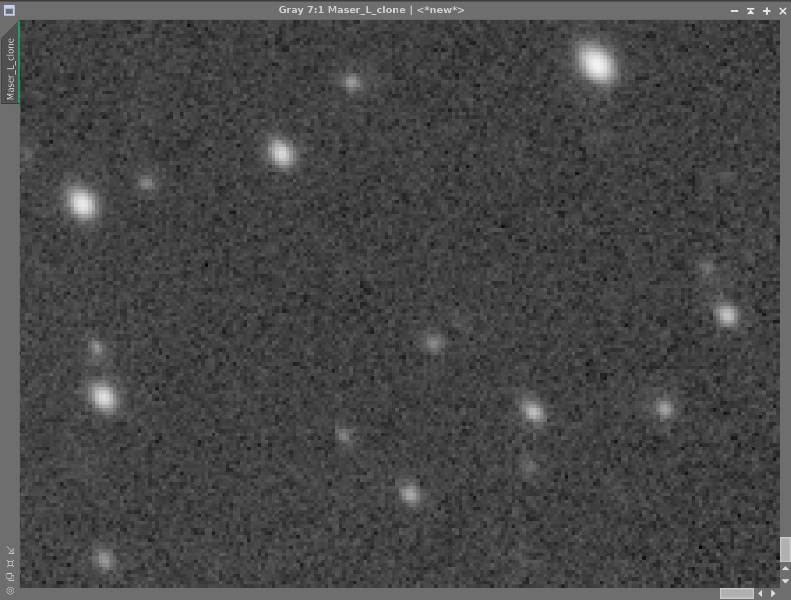
My Askar FRA400 platform has slightly undersampled data, so I pulled up a luminance frame from one of my projects and picked an area that also has a nice sample of two stars that were very close together.

A section of a Lum Master image from my Askar FRA400 platform. Note that the fainter stars are a bit undersampled and blocky, and also note the bright star towards the center that has a very close and overlapping companions star.

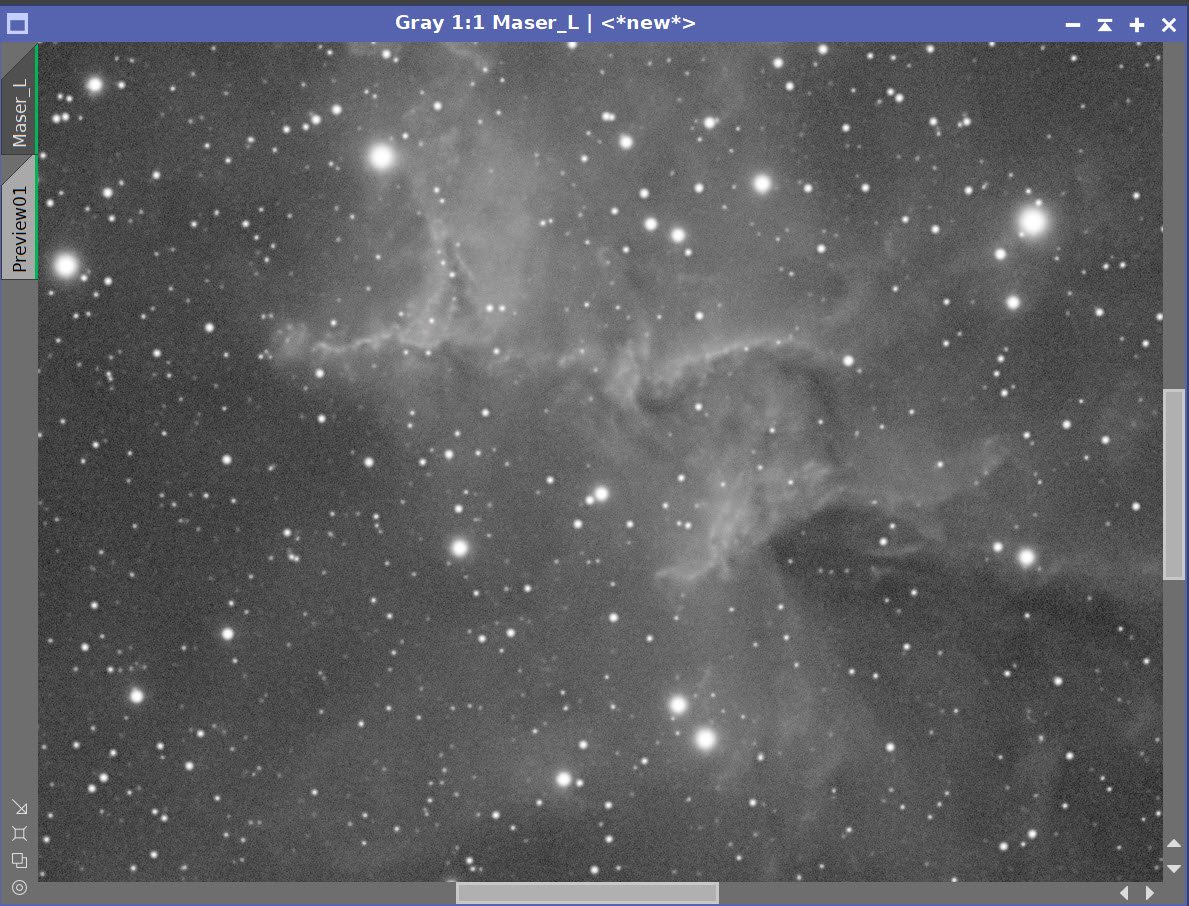
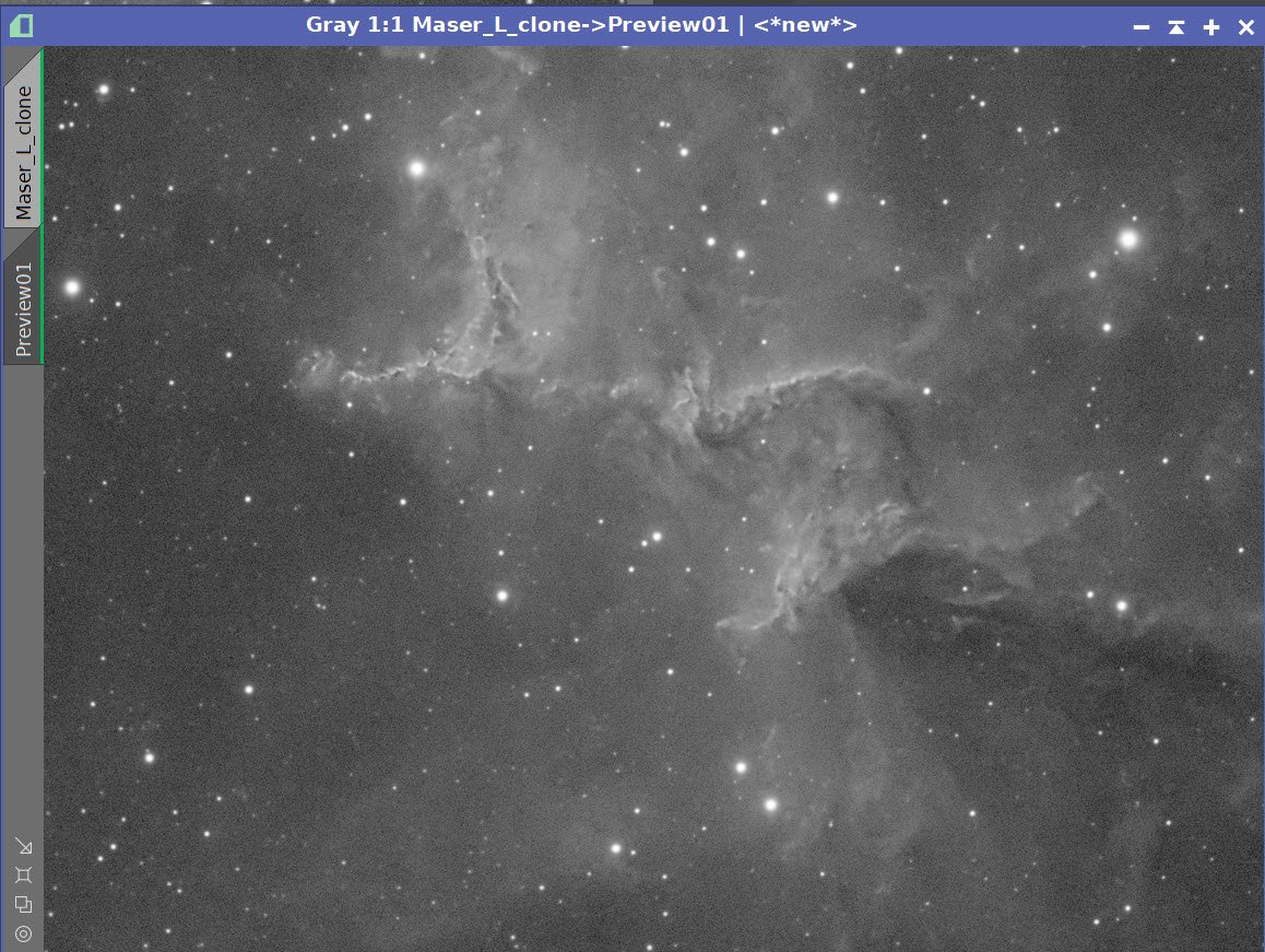
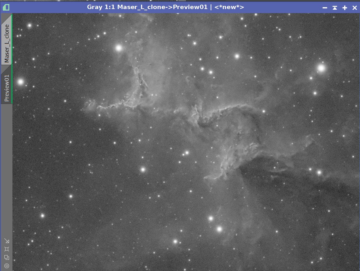
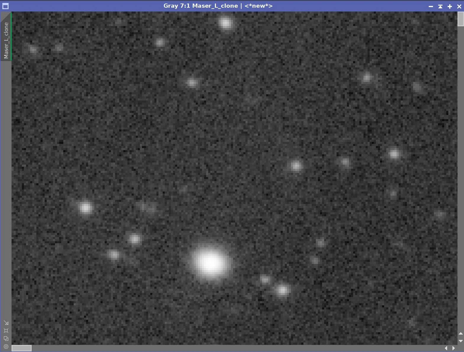
Here is after BXT was run with the defaut parameters.
After BXT was run, we can see that the overlapping stars seemed to be handled quite well! We can also see that the fainter stars, which are undersampled, came back as sharpened blocks.
This is no worse than I have seen with traditional deconvolution.
I think this shows that:
BXT does better when better data is provided to it
Just like traditional deconvolution, it really wants well-sampled data
One wonders if RC Astro could begin to improve the undersampled case in the future.
BXT Compared to Pixinsight Deconvolution
So - now let’s compare BXT to the normal deconvolution method.
The effort (time) saved through the use of BXT:
No need to create a separate PSF file.
No need to create an object mask or iteratively tune regularization parameters to protect low signal areas.
No need to create a Local Deringing Support Image
No need to Iteratively set deconvolution parameters to get a good result and avoid artifacts
Fewer and more intuitive controls to set
The power of BXT over normal Deconvolution:
It can correct stars distorted by the effects of guiding, aberrations, and coma
It can deal with PSFs that truncated or distorted
If creates and uses a differential PSF across the frame
It can operate across color channels, dealing with chromatic aberrations and other color artifacts
It provides greater user control over the processing of stars, halos, and nonstellar details
The downside of BXT?
It cost $100. This is fairly costly. On the other hand, it does an amazing job. Given my current investment of time and resources in astrophotography, I had no problem justifying it.
It is slow. Image of Luminance image of Melotte 15 took 5.5 minutes to run on my Ryzen 9 3900X 12-core CPU. 5.5 minutes is a long time to wait - but nothing compared to the hours I spent doing deconvolution with the old methods
It is not completely robust - inappropriate parameter settings can still cause artifacts.
May not be suitable for scientific work
if you take great pride in your ability to use traditional deconvolution, your ego may take a hit
You may need to change your workflow to maximize the final quality
So, in summary, BXT is easier and faster to use, has superior capability, and produces great results that are easy to control!
“Shut up and take my money!”
Workflow Considerations
Below is my current preferred Narrowband SHO workflow:

When using this workflow, I create a synthetic luminance image which I process to maximize sharpness and detail. Therefore, I tend to do deconvolution on the Lum image and fold this sharpness into the color SHO image using the LRGBCombination tool.
I could keep this workflow and continue to apply deconvolution with BXT on the Synthetic Luminance channel as I have been doing. On one level, I think this would be fine.
However, BXT does cross-channel optimizations. We’ve already seen one example where BXT was producing a superior result when it was able to operate on a color image and optimize how the three channels are processed. One Caveat made by Russell here is that BXT will do best if a pure SHO mapping is used. If the narrowband mapping uses blends of filter data (i.e. R channel is mapped by some mix of Ha, O3, or SI), a hybrid PSF - for that blend - will be seen and used. Since each filter will see star sizes differently - this can cause a less optimal result.
Since it looks like there is an advantage to doing deconvolution on a linear color image, I am contemplating changing my high-level workflow to something that looks more like this:

In this case, I would create an early version of the SHO image in the linear domain, run BXT, and then create the luminance image from this color base image. More testing will be needed to confirm this approach, but this is my current thinking.
When dealing with LRGB data, my preferred workflow looks like this:

In this case, we already have a color RGB image in the Linear domain, as well as a Luminance image. I could run BXT on both images and keep the rest of the workflow the same.
One Caveat here is if the sharpening level of the stars turns out different for the Lum Image compared to the RG image, you could get star artifacts when these images are combined with the LRGBCombinaton tool. Compare the sharpening output for the Lum and RGB images and just one to match the other the best you can to avoid this problem.
Once I have enough projects under my belt using BXT, I may find a reason to modify this, but this is what I will be doing as we move forward:

Workflow Caveats
Russel indicated that BXT should be used before noise reduction is done, as noise reduction can distort the low-contrast signal that deconvolution works on.
It is also recommended that PCC or SPCC be applied before BXT is run. Running BXT first will cause a broader point spread and different correction slopes that are not optimal.
So - What is a Neural Network?

Let’s Look at the Technology that BXT Uses.
The brain itself inspires Neural Network technology. We think of the brain as a network of neurons that are connected. We think of one neuron firing and triggering other neurons that are connected to it.
In the software sense, think of a neuron as a node that can hold a number between 0.0 and 1.0.
That node is activated if the number is high.
Neurons can be connected to many other neurons, and their current activation is based on the sum of the signals coming from those connections.
Now think of these neurons as stacked in a column. We can begin to build a network by starting with two columns of neurons.
The LEFT column is a representation of the inputs to the network
The RIGHT column is a set of outputs for the network
The number of nodes in each column is related to what information you are trying to feed into the network or what kind of output you want the network to produce.
Each of these columns is a layer, and we can have extra layers between the input and output layers. These are called Hidden Layers.
The number of layers and neurons in each layer can vary greatly.
Adjacent layers are fully interconnected.

A representation of a neural network with three hidden layers.
This Classic form of network is called a Multi-Layer Perceptron or MLP.
Data is propagated through the network from left to right. Data is loaded to the input layer, and activations in the input layer cause activations in the next layer. Thus the input feeds forward through the network.
Connections between the neurons have a weight associated with them. To determine if a neuron in layer two is activated, we take the sum of all of the neuron values from the previous layer times their weight plus an overall bias for that neuron.
Neuron A2 = a1w1 + a2w2+a3w2…. + Bias
Weights can be seen as the strength of any specific connection.
Biases are the sensitivity of that neuron. A higher bias means less signal is needed to activate.
Weights can have any value, but we want our neurons to have an activation value between 0.0-1.0, so we need a function that will convert arbitrary weight sums to that range. A Sigmoid function is often used to accomplish this.

So the value for a particular neuron becomes:
A2 = Sigmoid(a1w1 + a2w2+a3w2….. + Bias)
A network can be considered a function:
Output =f (inputs)
In fact, it has been proven that a neural network can emulate any arbitrary function.
An Example
Let's look at an example problem to understand this better.
One classic problem often used to explore Neural Networks is recognizing handwritten numerical digits between 0-9. In this case, we can assume that we dealing with a 28x28 grid with pixel values between 0.0 and 1.0 that represents samples of handwritten numbers.

From Wikipedia
If you were to take the columns of this grid and put them end to end, you would have 784 input neurons.
You could then have ten output neurons representing the numbers 0-9. The neuron with the greatest activation would be associated with the recognized digit.

A Neural Network for recognizing handwritten digits with one hidden layer. Taken from HERE.
Let’s say we added two hidden layers of 20 neurons each (this is very arbitrary). Our network would have the following:
784+20+20+10=834 neurons
784*20+20*20+20*10= 16,280 weights
We plug in an image, calculate things forward and see which output neurons are activated - the highest value is the digit classification.
This describes the form and operation of the network, but Its functionality is completely dependent upon the weights and biases loaded into the network.
The secret, then, is in setting the right weights. How is this done? A learning process is used to accomplish this!
The Learning Process
Several components enable this learning process:
Training Data Set: This set of data consists of a large population that represents the input and desired outputs for a network. For a given input to the system, you also need the “right answer” you want the network to compute. You are telling the network that when you see this input data, you want to produce this output (also sometimes called the Ground Truth). This data will be used to drive the training process.
Evaluation Data set: This is very similar to the training data set, except that the network will never see this data during the training process. Instead, it is run through the resulting weight network to evaluate the performance of the network and to ensure that the response of the network generalizes.
A Set of Random Weights: The network is loaded with random weights. This means that before training occurs, the network's performance will be random and, therefore, terrible. But you have to start somewhere, and this defines a starting network condition.
Cost Function: Ths function compares the output of the network to the ground truth and computes a cost - which is really just a measure of error
You can get into much detail on how weights are changed during the learning process.
Suffice it to say for our purposes, errors are factored backward in the network in a process that determines how to nudge the weights into a direction that will help minimize the errors produced on the last run. We start at the output nodes and work backward on the weights feeding directly to them. Then we work backward further - to the next layer- determining which weights if changed, would have the best result in reducing the system's error. This process is called Back Propagation learning.
One cycle will nudge things around such that the network will do a slightly better job. You will need a lot of cycles in order to complete this “nudging” process.

Training consists of finding the lowest error in a two-dimensional space. In practice, we operate with many more dimensions, but the two-dimensional example is easier to understand.
In our example, we have a 20-neuron hidden layer feeding into one neuron of the output layer. This is like having 20 weighted measures that, when summed, will provide the final answer for that output node.
This is a 20-dimensional space, and the task here is to nudge the weights such that we move along an error surface mapped in this space and try to find the lowest point. This method is known as Gradient Decent. This involves some sophisticated calculus and is hard to envision because the human mind works best with only three dimensions.
So training means we:
Run through the training set and produce a set of results
Compare the results to the desired aim and calculate the cost function
Use Back Propagation Learning to nudge the weights feeding each neural in the right direction to reduce the cost
Repeat. At some point, the weight changes become so small that learning converges, and the process is done. This can take a LOT of computer cycles to accomplish.
Once our learning is complete, we can run our evaluation data and see if the result generalizes across broader data sets.
My First Exposure to Neural Networks
This then describes, at least a high level, what a neural network is.
Back in the 90s, I worked at Kodak R&D on creating a class of algorithms called Scene Balance Algorithms, or SBAs.
A Scene Balance Algorithm was used in high-speed film printing systems to map the right point in the large dynamic range of a color negative onto the narrower range of photographic paper. Basically, it determined what exposure was needed to make sure that the main subject of the image looked good when printed. Before the advent of SBAs, trained operators looked at the negative and pushed correction buttons to get the right results. But operators are slow and tend to want to get paid for their work, so our job was to replace the operators with an automated algorithm.
A film scanner would look at a frame of color-negative film and the SBA would compute the right exposure point so that when printed, an image had the right neutral and color balance.
At the time, this was done with stepwise regression analysis, creating between 9 and 12-dimensional linear and nonlinear models that would predict the needed exposure levels.
The trick here was to have a population of color-negative films that represented consumer image-taking habits. These populations had thousands of frames, and each would be printed by hand until the results were as good as we could get. This was our training population. We have the scan data for each image and the aim exposure times needed to make a good print.
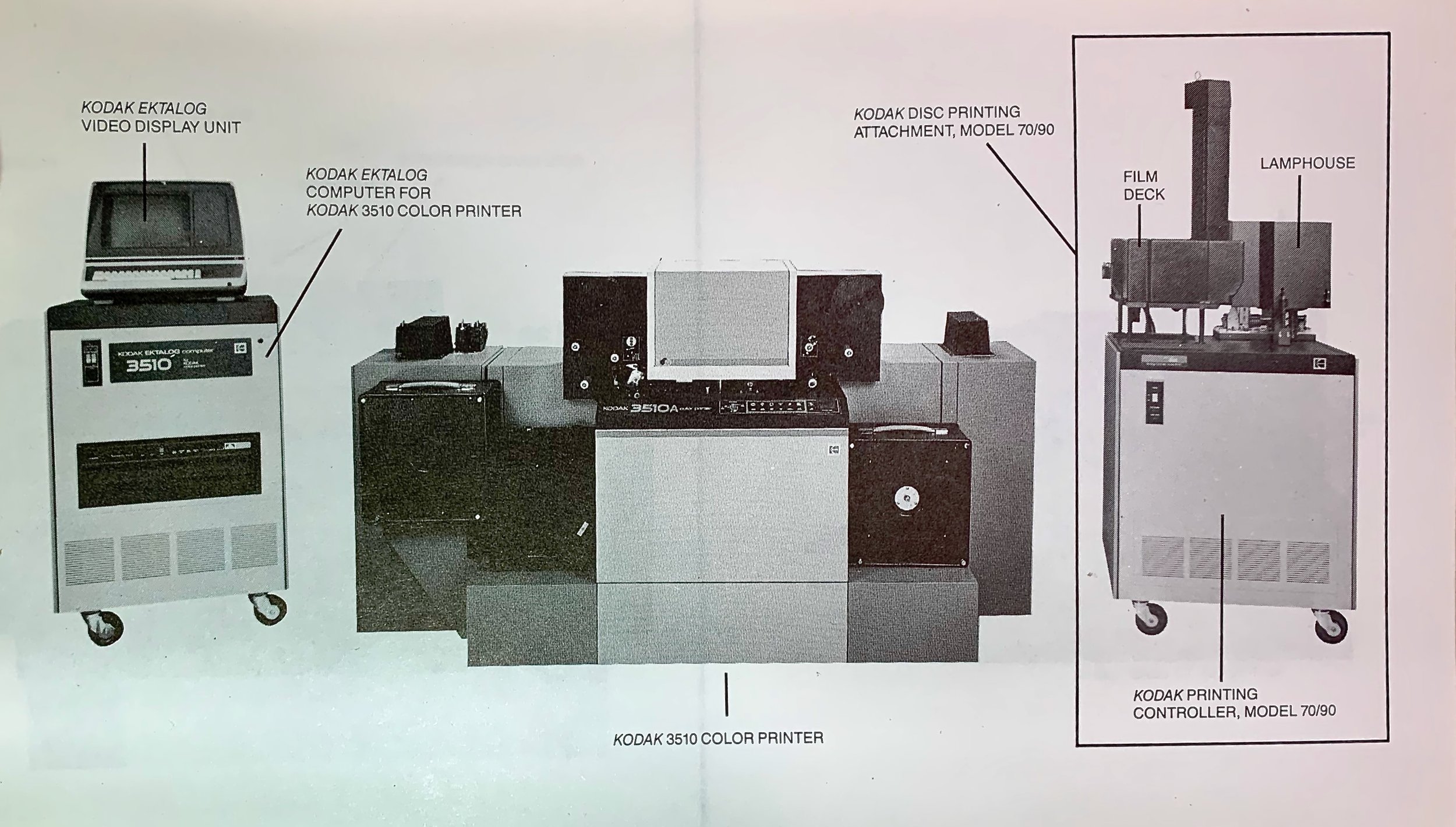
The Kodak 3510 Color Negative Printer. This was a high speed optical printer that used a low resolution 10x7 color scanner to analyze frames and use automated algorithms to expose the paper to make prints. I worked on the models that were used to drive this.
We would then calculate a series of over 100 predictors computed from the scanned negative data. Each one represented some characteristic measure of the image. We would then do a stepwise regression analysis to determine which predictors created the most useful N-dimensional model with the aim data. This model was then used to automate high-speed photographic printers.
These predictors were used because each represented some kind of unique measure of the negative. In those days, our film scanners were very low in resolution. Some have only a 10x7 scan grid in R,G, and B colors. Another had a resolution of 24x36 pixels in three colors. While low in resolution, this information told us much about the scene we were dealing with—Minimum Densities, Maximum Densities, Average Densities, Center Versus Surround Densities, etc.
Loading each pixel value into the regression made no sense. For one reason, there were too many values to deal with at the time. For another - many of the pixel values in a common region were similar, meaning the dimensions defined by these pixels were cross-correlated - which was a bad thing when doing least-squares-based modeling.
So the predictors were an attempt to extract a set of features from the image into a smaller set of measures that tended to be orthogonal from each other. Think of the predictors as a set of measures that describe the essence of an image with a kind of shorthand.
Stepwise Regression would explore a set of 100 possible predictors and narrow it down to a small number used to create the final model. Often these models only used 9-12 predictors - these seemed to boil down the essence of the image from the large pixel data set.
Where Neural Networks Come In
I was also working on my Master of Computer Science at the time, and I was introduced to Neural Networks.
I quickly realized that I had perfect training data for such a network: over 100 hundred predictors and one aim. I also realized that a neural network could emulate a linear or nonlinear model in that space.
What if I could create a neural network that was more successful than regression was?
So I wrote the code to implement neural networks and code to do the training. I trained the data for weeks. My cost function was squared error - just as the regression used. Ultimately, I came up with a network with significantly lower errors than any regression model I had ever created. I was very excited by this result. Then I ran my evaluation data set, and the results were not as good! The response of the neural network did NOT generalize. Apparently, the training data had to be a much larger data set than we could logistically create at the time.
But this exposed me to the concept of neural networks. They were a fascinating construct - and they worked so differently than regression analysis that I found the whole concept just fascinating.
That was a long time ago, and since then, neural networks have evolved into much more sophisticated beasts.
Convolutional Neural Networks (CNNs)

Animation of running a kernel across an image.
When we think about neural network working on Astro images, we run into an informational problem.
A typical Astro image might be 2k x3k in size and have three color layers. That would mean we would need an input layer of 2K x 3K x 3 colors, or about 18 million nodes! If I want to predict what the output image is, I would need another 18M out nodes. This would get hairy fast.
We would also run into the same problem that I had when working on SBAs - the raw data was redundant and cross-correlated.
Then along came Convolutional Neural Networks. These add extra hidden layers that reduce the amount of the image data being dealt with. These layers allow features to be extracted from the raw data, which can hold semantically useful data for the problem being solved.
These hidden layers take three forms: Convolutional, Pooling, and Fully Connected.
The Convolutional Layer runs a kernel of some size (say 3x3 or 5x5, for example) over the image and extracts feature maps of the starting image. The features extracted are defined by the different kernel definitions.
In many ways, this was similar to what I used to do with my old regression work. I could not deal with all the raw pixels, so I created a set of feature extractions - which for me, was a set of predictors. This reduces the key data in the network and tends to concentrate on the semantic aspects of the image.
The pooling layer simply reduces the resolution of the input layer.
The Fully Connected Layer is the kind we saw with a traditional neural net, where nodes between layers are fully connected.
It is not unusual to have a set of convolutional feature extraction layers that are then pooled. Then another set of convolutions and pooling occurs again - dramatically reducing the data load while preserving key information content.
CNNs are extremely well-suited for imaging applications.
They are many forms of CNN architectures.
Some are set up for image classification problems. These start with full images as inputs, and the output is some classification codes. These are often described as CNN + MLPs:

Taken from the publication HERE.
These tend to reduce the raw input data into a set of useful features that are used in the network to do some form of discrete classification.
Some are set up for image transformation problems - with a full image as input and a full image as output. Some of these are brute force, going from a full-resolution input image to a full-resolution and transformed output image.
Some boil the image down into key features and codes - and then regrow the image from these descriptors.
Some break the image into tiles and process the smaller tiles and build the image back up, one piece at a time. To minimize discontinuity between the tiles, the tile is overlapped by 20% or more.
There are a lot of possible architectures that have been created for CNNs, but all typically build with a combination of convolutional layers, pooling layers, and fully connected layers.
Let’s look at some examples of these:
Vanilla CNNs:
These are networks that consist of just convolutional layers. These can retain the input resolution and have been used for image restoration applications.

Vanilla CNN - Taken from the publication HERE.
ResNets
ResNets consist of groups of convolutional layers that can compute image residuals. They often contain Skip Connections that add earlier version layer results to later layer results. They have been used in image refinement.

Taken from the publication HERE.
Encoder-Decoder Nets
Encoder-Decoder Nets use convolutional layers to create critical feature maps that allow the images to be described by a shorthand code that takes up much less space. This is referred to as Encoding. This reduced size representation forces the learning of image semantics. This code can then be reconstituted back to a full res image with the Decoder section, including desired transformations.

Taken from the publication HERE.
Autoencoder Net
Similar to the Encoder-Decoder, also known as a UNet, this network architecture allows for unsupervised learning and has been used for noise reduction applications.
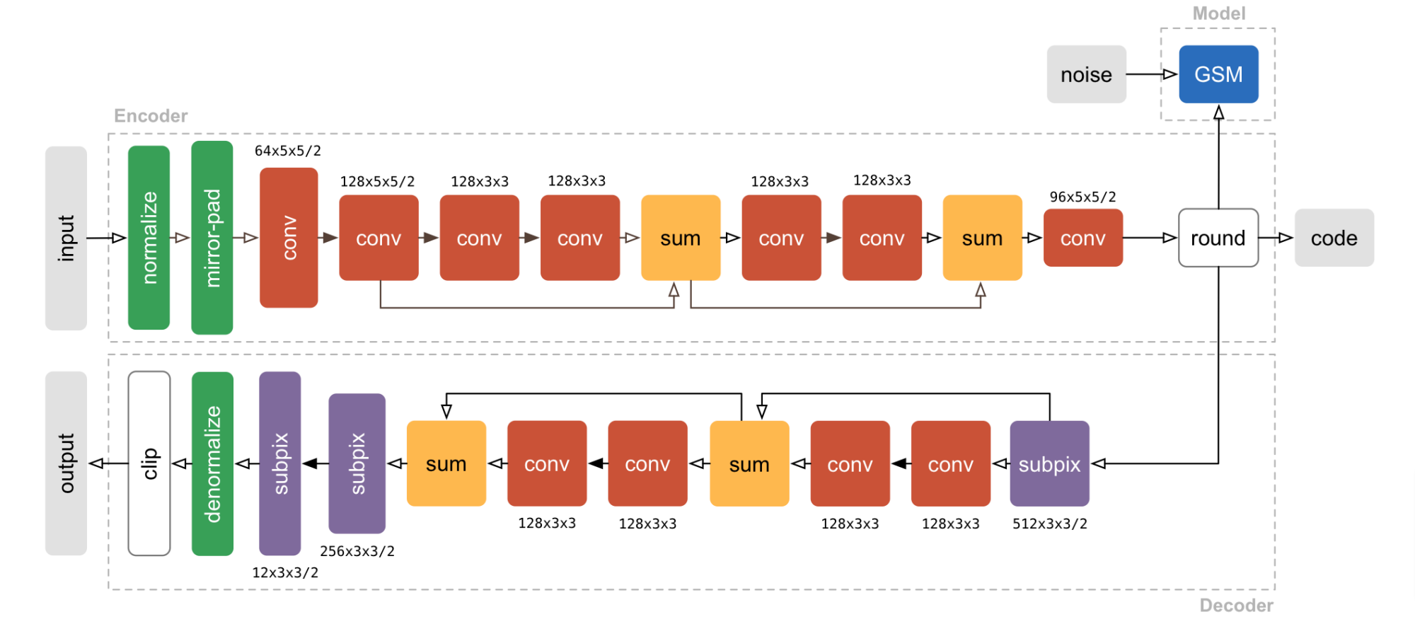
Taken from the publication HERE.
Summary
Muli-Layer Perceptrons, or MLPs, represent a set of fully connected layers of artificial neurons in a feedforward network whose weights can be set by a training process.
Convolutional Neural Networks allow the addition of hidden layers that extract features from the input layer and can reduce the data used while raising the semantic knowledge of that image. This makes Convolutional Neural Networks well-suited for image applications.
There are many architectures for CNNs that allow for various image transformations.
The final performance of these networks is based on the training done. This, in turn, is dependent upon the quantity and quality of the input and output training data, the design of the cost function, and having sufficient data that allows for testing for generalization.
Want to Learn More About Neural Networks?
Here are some great links that will help to dive deeper into neural networks and convolutional networks:
Neural Networks from the Ground Up - Chapter 1 Deep Learning, by 3Blue1Brown (Youtube Video)
Gradient Decent: How Neural Networks Learn - Chapter 2 Deep Learning, by 3Blue1Brown (Youtube Video)
What Is Backpropagation Really Doing? - Chapter 3 Deep learning, by 3Blue1Brown (Youtube Video)
Neural Networks and Deep Learning - Free online book by Michael Nielson
A Comprehensive Guide to Convolutional Neural Networks — the ELI5 way - by Sumit Saha
De-Blurring images using Convolutional Neural Networks along with code, by Anurag Pendyala
Neural Network Architectures for Images by Paul Hand (Youtube Video)
So, What is RC Astro Doing?
We don’t really know. I certainly have no insider information.
There are some hints from the documentation provided.
I believe BXT is based on one of the forms of CNNs. There are published papers on the use of Autoencoders for the purposes of noise reduction. Since RC Astro has already released NoiseXTerminator, I could imagine a scenario where the Autoencoder model was followed for that application. Then, based on learning made there, deconvolution came next.
Obviously, they are using Astro Images as the basis of their training data. The documentation tells us that data from the Hubble Space Telescope and the JWST was used - but how?
First, they would need to get input data. One possibility could be using data from known objects taken from various telescopes and camera combinations. There are certainly a lot of images out there that could be leveraged for this. But how would you get your aim data?
You could run traditional deconvolution on all of this data and use that as an aim. But that might not be good enough for training superior performance. Plus, the logistics of running Decon on a large population of images seems unreasonable.
What if the Hubble and JWST data were used as Ground Truth?
Think about it:
Hubble and JWST images are in the public domain.
They do not have distortions due to atmospheric effects.
They do not have the tracking/guiding problems we have here on Earth.
The optics used are very high precision compared to the devices used by most Astrophotographers.
The optical distortions for each instrument are known and calibrated to a great degree.
Data from these sources have eliminated most of what deconvolution tried to correct for!
I could imagine that plate solving would allow data from Earthbound telescopes to be correlated with Hubble/JWST data. Input images tied to Aim output Ground Truth images!
Also, we know that BXT works with tiles that are 512x512 in size. Perhaps the training images are all broken into this size, and these smaller image samples are both the input and output of the system.
We also can surmise that some of the feature extraction has to do with stars. We know that RC Astro has this capability based on their superior StarXTeriminator. It’s not surprising that star features extracted from a 512x512 tile would allow for good measures of differential PSFs in an image!
Further, we know that this feature extraction would be a key enabler for deconvolution training.
Again - this is all speculation.
Clearly, Russell Croman has done a lot of work in the arena and has found a viable combination that allows BXT to work as it does!
UPDATE:
After this article was written, Russell Croman published a video on his Youtube Channel of a 2022 AIC Presentation he gave that covers his overview of Convolutional Neural Networks and how he does training. I wish I could have seen this excellent presentation before writing this article!
For the most part, I think I called things pretty well. He does appear to be using Convolutional Neural Network with extracted feature sets and poling in an Autoencoder architecture.
It sounds like I may have gotten the training data wrong, and my interpretation of what he said suggests that Hubble/JWST data was used for ground truth but then was convolved to get the input data. This begs the question of what PSF he was convolving with? It could well be that this convolutional kernel was based upon some average PSF seen in typical Earthbound Telescope/Camera combinations.
At any rate, I wanted to share Russell’s excellent presentation here for your consumption:
https://www.youtube.com/watch?v=JlSUVJI93jg&t=0s
What About All those Concerns About BXT?
Now that we know a little about the technology behind BXT, let’s revisit some of the concerns raised about it.
”BXT is replacing your pixels with some else pixels - it’s unethical and a form of cheating!”
This is from the Conspiracy Theory Crowd.
This just seems silly to me. Creating a Neural Network that would do a great job with deconvolution is hard. Still, a tool that could figure out what you are looking at, replace the data in your image, and do it in a way that is seamless and undetectable is way harder to do in my mind.
My guess is that people heard something about using Hubble Telescope data in training and were confused by what that meant. Yes, it was trained by looking at other data, but the result was a set of weights that defines a mathematical function. This function is now used on any new image presented to it, and the function transforms the image data in place - emulating the action that we call deconvolution.
This is exactly what you were doing before when you were running traditional deconvolution. You were running a function that transformed the image data. At the end of the day, this is just math.
By the way - if BXT is swapping out data - where is it getting all of this data? The cloud? BXT runs with no network connection. From the data files downloaded as part of the installation? No - not enough data there to handle all cases. No, this is just silly.
“This technology is leading to one-button fixes - which will kill astrophotography.”
This, I think, is from the Sour Grapes Crowd.
Personally, I think this kind of correction is still very far off and not at all trivial to do using deep learning technology.
I have always maintained that if you gave the same image data to ten different astrophotographers and asked them to process that data - you would end up with ten excellent images that all look VERY different.
So think about the training data you’d need: You have one set of inputs and hundreds of different-looking aim data sets that are all valid outputs. Sounds like a training nightmare to me.
This technology is suited to solving one well-defined problem at a time.
We have seen it do well with star removal, noise reduction, and now, deconvolution. I don’t know about you, but it takes me days to process my images, and Star Removal, Noise Reduction, and Deconvolution are just a few steps among hundreds of others. Most of these other steps have a much greater impact on the final visual look of my image.
If I had a one-button fix - I would insist on having controls that would allow me to modify how it worked so that I produced images that met my artistic vision for these images.
I really don’t see this as a serious concern.
“BXT encourages sloppy data collection.”
I can almost see this one. Why get a field flattener if BXT can fix it? Why worry about how good your guiding is if BXT can fix it? And so on.
If you end up with those problems on a data set you have collected, having software that can minimize those issues are a godsend.
But I don’t really see something like BXT as being a crutch. We will find that the better our data is, the better the result will be from BXT. Dedicated astrophotographers move down a learning curve where they begin to pay attention to smaller and smaller details and effects. They realize that creating a great image requires the summation of many small details. I don’t think this will change. I think the old garbage-in/garbage-out adage will remain true to an extent, and great astrophotographers will always strive for the best data and processing they can achieve. I don’t see BXT changing that.
Better data will always yield a better image.
“I don’t really know what this mysterious AI is doing, but it just seems wrong.”
Starnet, Starnet2, StarXTerminator, NoiseXTerminator, and the Topaz suite of tools all use the same technology approach, and I never hear a hint of concerns there. Why are we hearing it now for BXT?
My guess is that you have some people who were proud of their accomplishment in mastering deconvolution and just don’t like the idea that someone who has not mastered this skill can now get better results.
I suppose this is nothing new. I imagine that when autoguiders first came out, there was a group of accomplished manual guiders that were not at all supportive. Or when the first digital camera replaced film cameras. And so on. For me, it just lets me spend more time working on other problems.
The fact that you don’t understand the technology does not give you a license to make stuff up and let your beliefs swamp reality. I recently saw a post along these lines from a YouTuber with a significant following. I won’t name him here. I posted this response to him:
You have presented a fundamental misrepresentation of what BlurXterminator does and how it does it.
BlurXTerminator is a standard AI network trained by presenting example Astro data with a scoring function for good and bad results. Iterative training is done so that the final result is a weighted network representing the functionality "learned" by seeing example data. It is trained on other data from other images - but it does not use other data from other images to replace data in your image.
It is the same methodology used to create NoiseXTerminator and StarXterminator - and there has never been any real controversy there.
It is the same technology used to develop the Topaz products - but in that case, the training data was standard pictorial images, not dedicated astro images - so it does not work as well for our application and can cause artifacts.
The AI network represents a deconvolution function that is more powerful than the standard deconvolution function, as the PSF it creates is differential across the frame of the image. Plus the method can deal with truncated and distorted PSFs, which the standard method cannot do. Further, it can modify the PSF used based on the local distortion as seen in stars found in that local region. So it is a better and more adaptive way of deconvolution - and therefore more accessible by beginners. It also provides simple controls that allow you to determine how much of the deconvolution effect will be applied to star cores, star halos, and non-star structures.
That is pretty cool and allows astrophotographers a great deal of control over how it improves their images. It does not copy data from other images or access any catalogs in the cloud. That is just plain silly. All this tool does is deconvolution. This is a tiny portion of the complete processing an image goes through and certainly is not a push-the-button and out pops a perfect image. It just provides an alternative and frankly superior way of doing deconvolution, which can restore some lost sharpness in an image during the capture process.
If you have good data, your image is improved more than if you have bad data. So this does not suddenly dispense with the need to go after quality data.
There may be some that prefer to use the standard method of deconvolution. If you know what you're doing there, you can get excellent results. If you prefer that method to this new one, then don't use the new one. But to claim this tool is doing something it is not doing - and then cast shade on it based on that misrepresentation - is simply not accurate nor is it fair.
To his credit, he recognized that he had inaccuracies in his video and took it down.
There may be some that just don’t like BXT. Perhaps they enjoy the process of using the old method. Perhaps they feel they have more control over the old method. Perhaps they just don’t yet trust the tool. I have no problem with this. At the end of the day, a deconvolution is just a tool, and if you prefer one tool over another - have at it!
Conclusion
The traditional deconvolution found in Pixinsight is a tool that can only be used by those who have learned to master its complexity and are willing to invest the time and effort needed to yield good results.
Russell Croman Astrophotography has used deep learning technology to create a breakthrough tool that changes all that!
They have created a tool that requires little special knowledge and no prior preparation to use. A tool that is more robust and easier to work with. A tool that has superior performance.
It is a game changer. It has changed how I will do image processing as I go forward!
Something that solves a big problem reduces the effort and time needed, and intuitively produces excellent results should be welcomed!
So, in summary, I would say:
"Remember my 9-part deconvoution series ? Well just forget all of that crap and buy BlurXTerminator. The End"