
Melotte 15 - The Heart of the Heart Nebula (IC 1805) - 5.5 hours of SHO
Date: Nov 18, 2022
Cosgrove’s Cosmos Catalog ➤#0115
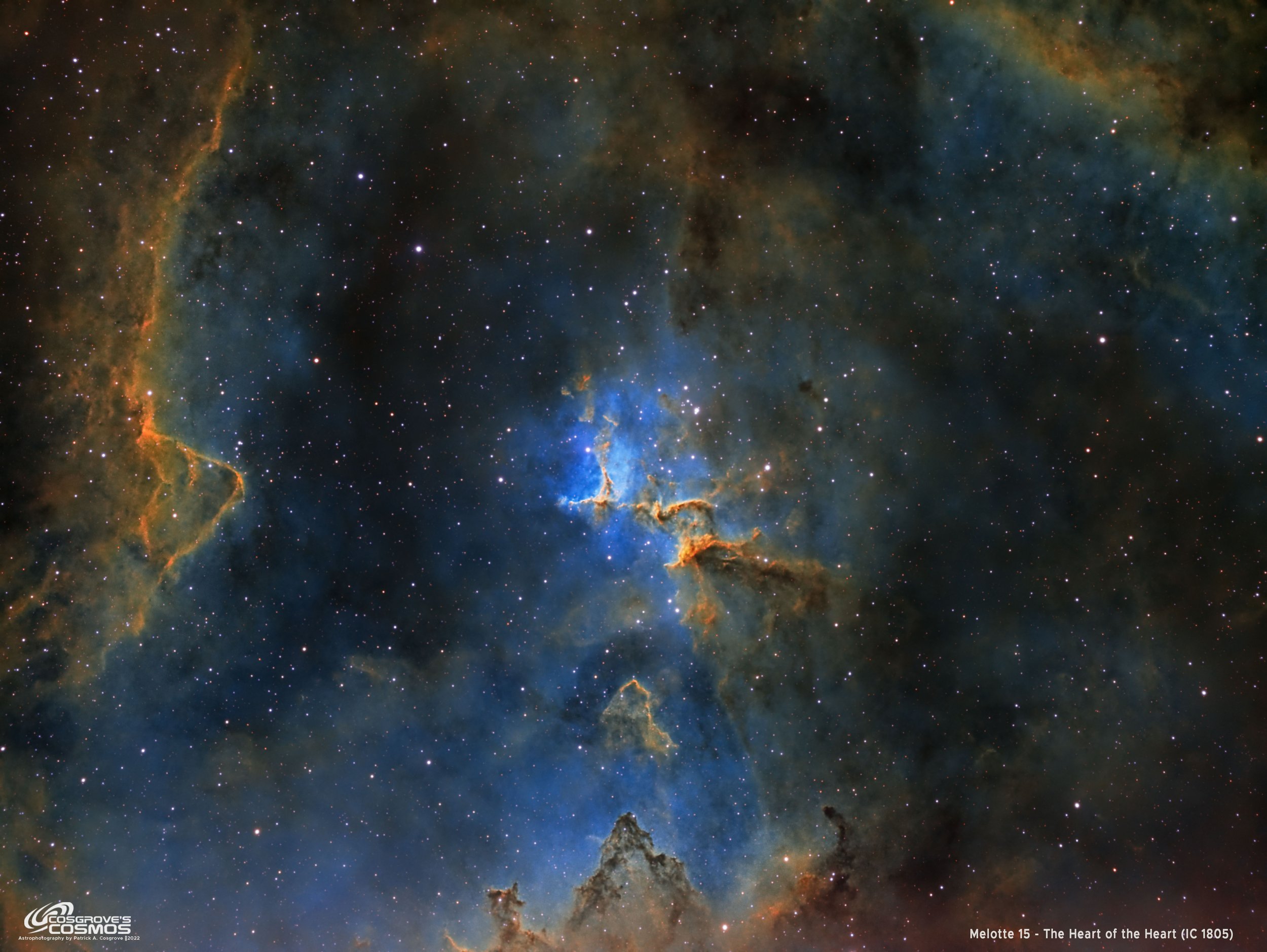
Melotte 15 - the Heart of the Heart Nebula (IC 1805) (click for high resolution version via Astrobin.com)
Awarded “Explore” Status on Flickr!

Table of Contents Show (Click on lines to navigate)
IC 1805 - The Heart Nebula - showing the location of Merlotte 15 outlined in yellow. (click to enlarge)
About the Target
IC 1805 is better known as the “Heart Nebula.” It is also known as the “Running Dog Nebula”, and Sharples 2 -190. It can be found 7,100 light-years away in the constellation of Cassiopeia. This a region rich in gas and dust and newly formed stars.
Towards the middle of this object is an open cluster and nebulae known as Melotte 15 - it is also known as Collinder 26, and sometimes called the “Heart of the Heart.” The open cluster contains a few stars that are larger than our own Sun - some as much as 50 times larger! It also has many stars that are just a fraction of the size of our Sun.
It was discovered by William Herschel on 3 November 1787.
Wikipedia tells us that:
the Melotte catalogue is a catalogue of 245 star clusters by British astronomer Philibert Jacques Melotte. It was published in 1915 as A Catalogue of Star Clusters shown on Franklin-Adams Chart Plates.[1] Catalogue objects are denoted by Melotte, e.g. "Melotte 20". Dated prefixes include as Mel + catalogue number, e.g. "Mel 20".[2]
The Annotated Image

THis finder chart was created with the ImageSolver and FinderChart tools in Pixinsight.
The Location in the Sky

This annotated image was created using the Pixinsight ImageSolve and ImageAnnotation scripts.
About the Project
Intro Video
A few minutes of introduction for this project by yours truly! While the processing walkthrough at the end of this post is quite detailed, sometimes it is hard to determine why some steps are done in the sequence they are. I wanted to find a way to have a 50,000-foot view and get a sense of the forest versus the trees.
In this video, I also cover the experiment I tried with creating an aggressive detail enhancement of the L-Starless image and compared it to a more selectively processed L-starless image.
Choosing the Target
This is the third target I have processed from my capture session in late October.
I was away from home for a few weeks with plans on returning home just in time to start the next capture cycle. With longer nights, I had planned on capturing two waves of targets for each scope - and I made my plan accordingly.
As I looked for what targets would be well positioned for me (and my tree line), I saw that the Heart Nebula would be within reach from about 1:45 am until about 5:30 am. I was still looking for something I could shoot later in the evening with my William Optics 132MM FLT platform, and I thought about The Heart Nebula. The problem was that the William Optics scope has an image scale large enough that there was no way I could fit this target into its field of view. In other cases, I have found some areas of interest in the larger target and focused in on that portion. Melotte 15 is an interesting area located right in the middle of IC1805, and I thought this would be a great target to go after. I used SGP’s Mosaic and Framing Wizard to dial in a nice composition, and I was ready to go! I planned to go for up to four nights of data capture.
If you have seen the post for my previous two projects, then you know that I came home from my trip with a very bad cold. This cold worsened during the first two nights of capture until things got really bad for me. It evolved into the worst respiratory and sinus infections that I think I ever had in my life.
It was so bad that everything just stopped - for weeks.
This cost me two beautiful clear nights when I could have captured more photons - but that was just not in the cards!
Data Capture
Subs were captured over the nights of Oct 21 and 22.
In general, these nights were clear and cool. The first night was a bit breezy, and I was concerned about my guiding given that my scopes are in the driveway and exposed - but the guiding stats looked good, and the subs showed good star images. I did not think either night was particularly transparent - but my subs seem to be looking reasonable, and I was satisfied.
Data Analysis
Blink analysis showed that the data looked pretty solid for all filters. No subs needed to be removed. I ended up with just shy of 5.5 hours of narrowband data. This was not the deep integration I had hoped for, and because of this, I did not feel I was in a position to use SubFrameSelector to identify outlier frames and cull them, as I often do. In fact, I skipped this step entirely and trusted the rejection logic to help me here.
Previous Efforts
I have never shot Melotte 15 before, but I have shot IC 1805 - The Heart Nebula - once before, about a year back in November of 2021. That was a deeper 11.5-hour narrowband integration that I thought came out quite nicely.
You can see that project posting HERE. You can see that image below - along with the current one, for comparison.
IC 1805 - taken in Nov 2021(click to enlarge)
Melotte 15 - our curren image (click to enlarge)
Image Processing
This project, just like the last few, is an SHO narrowband capture with 5-minute subs. It should be no surprise that I am using the same basic processing workflows and strategies for all of these images.
The basic flow is as follows:
Use a synthetic luminance image
Create the image
Process into the starless and stars-only image
Enhance the image for sharpness and detail
Create an SHO image
Process the master images
Adjust one to another
Create a color SHO image
Process into a starless and stars-only image
Process the image for excellent color and low noise
Prepare the star-only image
reduce exposure to reduce star sizes
Combine images
Roll L-starless image into SHO image
Add stars back in

The processing flow for this project.
I did try one interesting experiment this time around.
The basic philosophy around the Lum vs. Color processing paths is that you optimize the Luminance image for detail and sharpness and then optimize the color image color and low noise. By themselves, the images each lack information that is contained by the other. In theory, folding the Lum image into the color image produces an image that is the best of both words. The resulting image inherits the detail and sharpens of the Lum image and the color and smoothness of the Color image.
And this is how it basically works out. But I started to wonder how far I could take things.
Let’s say I have a nice smooth color image - what if I folded in a Lum image that was very sharp and detailed - aggressively so? How would that work out?
On the other hand, what if I was more strategic in preparing the Lum image? What if I selectively enhanced only critical elements of the scene?
I used this image to try both approaches and see how they worked out.
I did some aggressive detail enhancement for the whole L-Stareless image:
I pushed the contrast to a higher point
I did Local Histogram Equalization at a small, medium, and large scale and applied it to the entire image.
I did some aggressive sharpening.
The resulting -starless image was very sharp and contrasty. I then folded this back into the color SHO image. The result was VERY sharp - actually way too sharp. The image seemed harsh and hard on the eyes.
I then took a different L-Starless image and processed this with a much lighter hand:
I did a light-tone scale boost
LHE was still run to enhance at small, medium, and larger scales, but a mask was used to target these operations only to certain areas of interesting image structure - the rest of the image was left alone
Sharpening was avoided in this image - and only done further toward the end of the image processing effort.
The result was very different and much more pleasing!
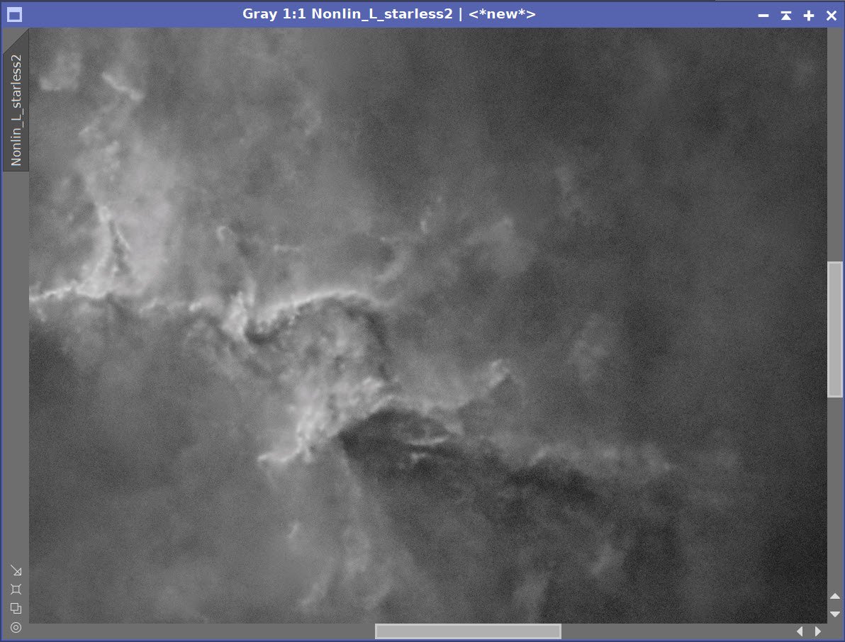
L-Starless after aggressive Detail Enhancement (click to enlarge)
L-Starless after more selective and controlled Detail Enhancement (click to enlarge)
Once these L-starless images were folded into the SHO color image, you could also see the difference come through:
Final image using aggressive L-Starless image (click to enlarge)
Final Image from more targeted L-Starless Image (click to enlarge)
While the high level of detail enhancement on the first image produced a final image that is very sharp - it is not as pleasing to my eye. It appears harsh, the background looks blotchy, and things just look unnatural to me. On the other hand, a more selective and targeted approach produces a very natural and pleasing image.
So you can take things too far! You always want the resulting image to appear natural.
Results
Given the fact that my integration is as short as it was, I am very happy with where the image ended up. The image has good contrast and drama, and the colors are deep without going too far. The noise is well-handled, and the detail level is pretty good.
With my last image, I was not sure if I really “loved” the results. No such issues here, as I am quite happy with the final image!
A detailed Processing Walk-Through is provided for this image at the end of the posting…
More Information
Wikipedia: IC 1805
Science.naa.gov: Melotte 15
Telescope.Live: Melotte 15
Capture Details
Lights Frames
Data were collected over two nights: Oct 21 & 22
25 x 300 seconds, bin 1x1 @ -15C, Unity Gain, Astrodon 5nm Ha
20 x 300 seconds, bin 1x1 @ -15C, Unity Gain, Astrodon 5nm O3
20 x 300 seconds, bin 1x1 @ -15C, Unity Gain , Astronmiks 6nm S2
Total of 5 hours 25 minutes
Cal Frames
25 Darks at 300 seconds, bin 1x1, -15C, Unity gain
15 Flats at bin 1x1, -15C, Unity gain - for Ha, O3, & S2 filters
25 Dark Flats at Flat exposure times, bin 1x1, -15C, Unity gain
Software
Capture Software: PHD2 Guider, Sequence Generator Pro controller
Image Processing: Pixinsight, Photoshop - assisted by Coffee, extensive processing indecision and second-guessing, editor regret, and much swearing…..
Capture Hardware:
Scope: William Optics 132mm f/7 FLT APO Refractor
Focus Motor: Pegasus Astro Focus Cube 2
Cam Rotator: Pegasus Astro Falcon
Guide Scope: Sharpstar 61EDPHII
Guide Focus Motor: ZWO EAF
Mount: Ioptron CEM 60
Tripod: Ioptron Tri-Pier
Camera: ZWO ASI1600MM-Pro
Filter Wheel: ZWO EFW 1.2 5 x8
Filters: ZWO Gen II 1.25” LRGB,
Astrodon 5nm Ha & O3 filters,
Astronomiks 6nm S2 filer
Guide Camera: ZWO ASI290MM-Mini
Dew Strips: Dew-Not Heater strips for Main & Guide
Scopes
Power Dist: Pegasus Astro Pocket Powerbox
USB Dist: Startech 8 slot USB 3.0 Hub
Polar Align Cam: Polemaster
Software:
Capture Software: PHD2 Guider, Sequence Generator Pro controller
Image Processing: Pixinsight, Photoshop - assisted by Coffee, extensive processing indecision and second-guessing, editor regret, and much swearing…..
Click below to see the Telescope Platform version used for this image:
Image Processing Walk-Through
(All Processing is done in Pixinsight - with some final touches done in Photoshop)
1. Blink Screening Process
Ha
Nice clear images
No trails or gradients
no frames removed
O3
Nice clear images
No trails or gradients
no frames removed
S2
Nice clear images
No trails or gradients
no frames removed
Flats
Flats were collected for each night. However, the flats for the second night looked dark and a little strange. So for this project, we will use the flats from the first night for both nights.
Dark flats
Looks good
Darks
300-sec darks all looked good.
2. WBPP 2.5.3
Load lights
Load flats first night only
Load darks - from the first night of bubble nebula
Load 300-sec darks
Select Maximum Quality
Keyword: Night
Output directory: wbpp
Set Dark Exposure tolerance: 0.0
Lights Exposure tolerance: 0.0
Enable image integration
Pedastal Image set to auto, set for all filters
CC set for all filters
Map missing flats and darks
Crashed during the first run!
16 minutes to run
Executed in 26 minutes - no errors

WBPP Calibration view.

WBPP Post-Calibration View

The new pipeline screen for WBPP version 2.5
3. Load Master Linear Images
Load the resulting Master Linear image and rename them.
Rejection High - Ha (click to enlarge)
Rejection Low - Ha (click to enlarge)
Rejection High - O3 (click to enlarge)
Rejection Low - O3 (click to enlarge)
Rejection High - S2 (click to enlarge)
Rejection Low - S2 (click to enlarge)
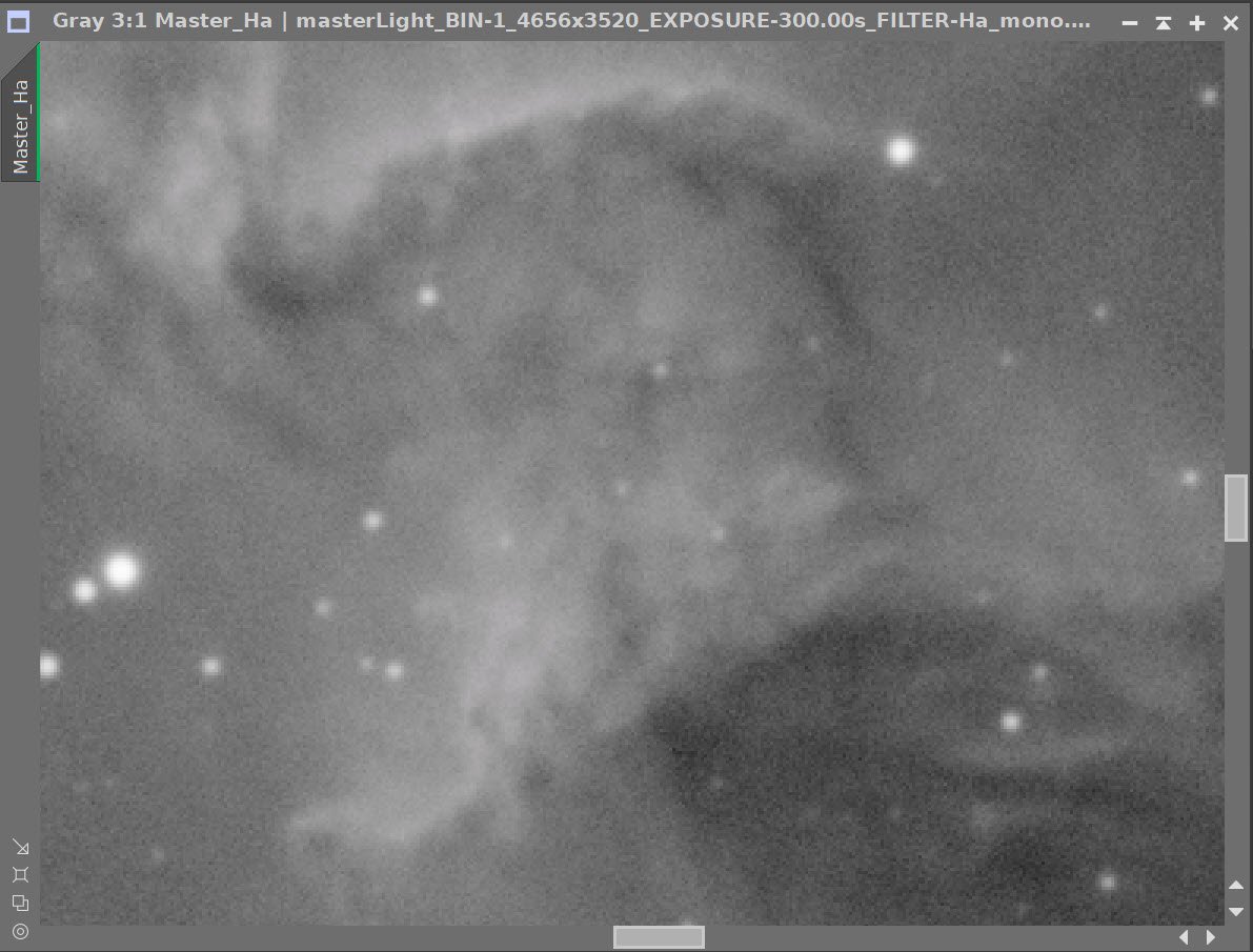
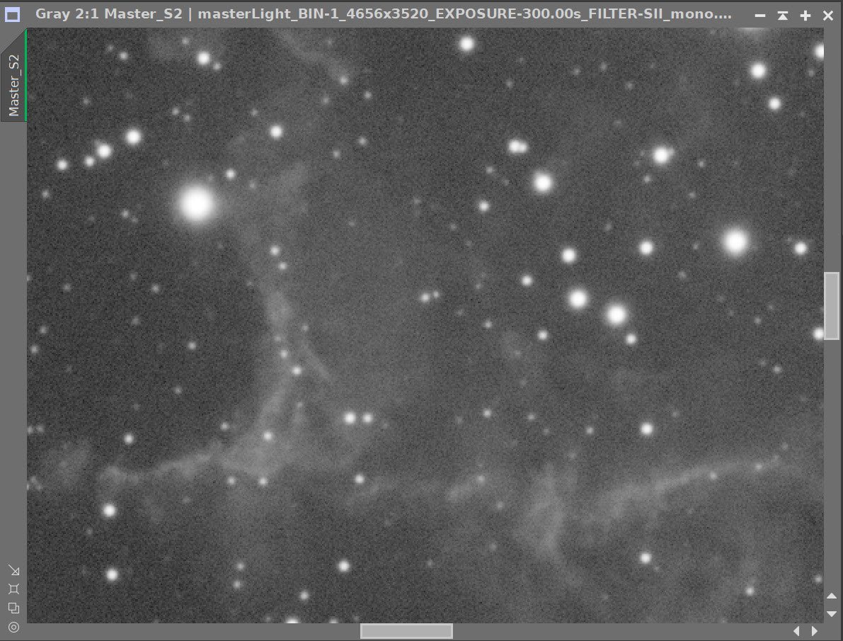
Master Ha (click to enlarge)
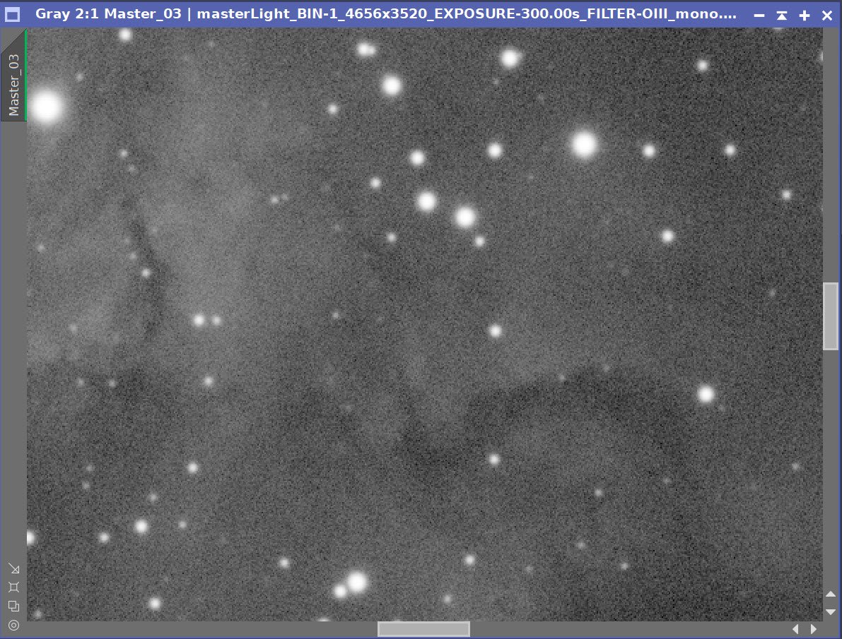
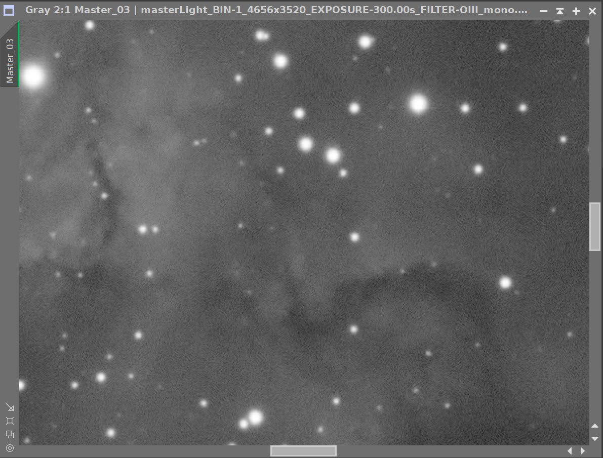
Master O3 (click to enlarge)
Master S2 (click to enlarge)
4. Crop all of the images
A common crop level was selected, and DynamicCrop was used to trim all of the master frames.
The edges were remarkably clean. Only a little had to be removed from the bottom edge.
5. Dynamic Background Extraction
I saw little evidence of gradients in these images, so I opted to skip the DBE step for this project.
6. Apply light Noise Reduction to the Ha, O3, and S2 Linear Master Images
A very light touch was used here.
Ha: Apply Noise XTerminator with a value of 0.4
O3: Apply Noise XTerminator with a value of 0.5
S2: Apply Noise XTerminator with a value of 0.4


Master Linear Images - Before and After Noise XTerminator
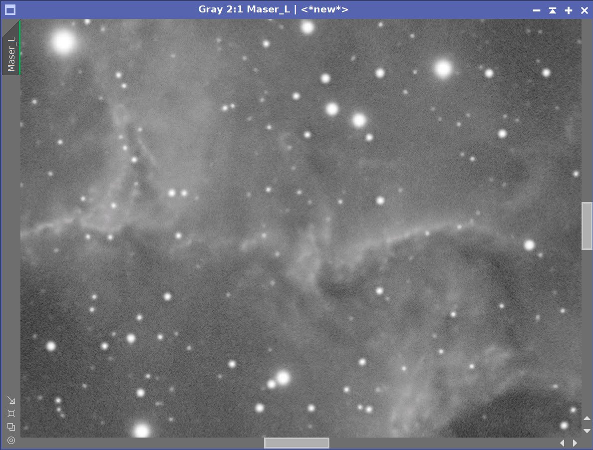
7. Create the Synthetic Lum image and Finish Linear Processing
We have three master images, which means we can use ImageIntegration to create the Synthetic Luminance Image.
I saved the 3 master images to disk.
I set up ImageIntegration to use those files, averaging for integration, and I disabled rejection.
Run and rename the new Luminance image.

ImageIntegration Panel as used to create the Synthetic Lum image.

The weights computed by ImageIntegration to combine the images

The computed Lum Image.

A 4-up panel showing the original and new computed L image for comparison.
Prepare for Deconvolution
Create PFS image using PFSImage script

The PFSImage Panel with settings used

The resulting final PSF image
Run Starmask to create the initial LDSI image (see panel snap for parameters)

The StarMask panel set up to create the LDSI map.

The HT tool was used in this config to boost the LDSI image
Compare the mask to the original image - the stars in the mask are too small to cover the stars in the image.
Apply HT Boost (see panel snap for parameters) 3 more times until star sizes match.
Checking the LDSI image against the Master L image - Star mask images are too small. (click to enlarge)
Checking again after apply 3 more levels of boost - sizes now look good! (click to enlarge)

The Final LDSI image
Select Preview regions on the image for Decon exploration

These preview regions were selected to iteratively test the decon panel parameters for optimized results.
Iteratively run decon on previews until parameters are finalized (see panels snap for final values)

The final Deconvolution Parameters are shown

Master L - Before and After Deconvolution
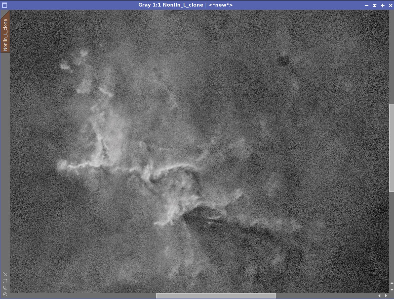
8. Process the Linear Master L Image: Option 1 - Aggressive Enhancement
Take the Lum image nonlinear using the MaskedStretch Process. Select a background preview and run the tool with default values
Do a final adjustment with CT.
The initial nonlinear L image after Masked Stretch (click to enlarge)
After Masked Stretch and a CT adjustment (click to enlarge)
Create a Starless Version of the image using StarXTerminator - creating a star image as well as using “Unscreen Stars”

The RC-Astro StarXTerminator Panel with settings used.
The Initial Starless L image (click to enlarge)
The initial Stars-Only Image (click to enlarge)
Apply CT globally
Enhance detail of the using Local Histogram Equalization (LHE). These changes will be applied to the entire image.
Enhance mid-scale detail with LHE radius=64, contrast limit=2, Amount=0.27, and 8-bit histograms
Enhance small-scale detail with LHE radius=22, contrast limit=2, Amount=0.15, and 8-bit histogram
Enhance larger-scale detail with LHE radius=300, contrast limit=2, Amount=0.2, and 10-bit histogram
After CT applied (click to enlarge)
Mid-Scale LHE enhancement (click to enlarge)
Small-Scale LHE enhancement (click to enlarge)
Large-Scale LHE Enhancement (click to enlarge)
Make a Lum mask by creating a copy of the L-Starless image.
Use HT to boost contrast and form an “object mask”
Soften the mask by applying Convolution with a stdev of 10
Apply a final CT
Apply the Lum mask and Invert it so that the background is exposed
Apply Noise XTerminator with a value of 0.8
Invert the mask
Apply MLT Sharpening (see panel snap below for details)
The lumnance mask created. (click to enlarge)
Lum Mask after Convolution (Click to enlarge)
Lum Mask After HT adjustment to create an Object Mask (click to enlarge)
Lum Mask after a final CT tweak (click to enlarge)

The MLT panel with the sharpening parameters used.


Masked Regions - Before & After Noise Reduction and Sharpening

Final Starless Lum Image created with aggressive global enhancement
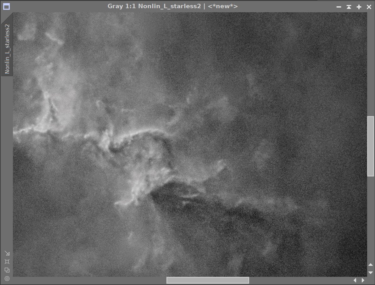
9. Process the Linear Master L Image: Option 2 - Selective Enhancement
Use the L-starless image after conversion to nonlinear space as a common starting point
Create a GAME mask that highlights and isolates the main structures of Melotte 15
Apply the mask and then enhance detail at various scales with Local Histogram Equalization (LHE)
Enhance mid-scale detail with LHE rdius=64, contrast limit=2, Amount=0.27, and 8-bit histograms
Enhance larger-scale detail with LHE rdius=300, contrast limit=2, Amount=0.2, and 10-bit histogram
Enhance small-scale detail with LHE rdius=22, contrast limit=2, Amount=0.15, and 8-bit histogram
Apply Noise XTerminator to the whole image with a value of 0.6
Apply a final tweak of CT
This will produce an image that is sharper in the most interesting details but also appear smooth and more natual.

Common Starting Point L-Starless Image
Game Mask to isolate key areas with interesting Structures (click to enlarge)
The GAME Mask in use showing coverage. (click to enlarge)
After mid-scale LHE enhancement with mask applied (click to enlarge)
Large-Scale LHE enhancement with maks applied. (click to enlarge)
Small-scale LHE enhancement with mask applied (click to enlarge)
Before and After Noise XTerminator

After final CT adjustment
10. Compare the two L-Starless Options
Option #1 is very sharp - but tends to look unnatural, and the background cloud details look clumpy.
Option #2 looks smoother and pretty natural with the main details enhanced
We will wait and see how these combine with the Color SHO image that we will create next
Option # 1 Aggressive Detail Enhancement (click to enlarge)
Option 2: More selective Detail Enhancement (click to enlarge)
12. Create and Process the Initial Color SHO image.
Take Master Images Nonlinear with the STF->HT method
Analyze images and tweak with CT to better match one to another
Use ChannelCombination to create the initial SHO image
Apply SCNR green 75% to reduce strong green case
Invert the image
Apply SCNR green 75% to reduce strong green case
Invert the image
Go starless using StarXTerminator - also, create a star map and unscreen the stars.
This will give us the option to use color stars later on if we want.

The original nonlinear images: Ha, O3, and S2.

After hand-tweaking the images.
The initial SHO color image. (click to enlarge)
Invert the image. Now magenta areas are green (click to enlarge)
After SCNR for Green. (Click to enlarge)
Apply SCNR for green. (click to enlarge)
Invert the image and adjust globally with CT. (click to enlarge)

StarXTermintor Panel
Initial Starless Image(click to enlarge)
The initial color Stars-Only Image (click to enlarge)
Create Color Masks with the Color Mask Script
create with -2 layers for softness
create Blue, Green, and Yellow masks
Boost each mast with HT
Apply Convolution with a stddev of 9
Apply Blue Mask and adjust with CT
Apply Green Mask and adjust with CT
Apply Yellow Mask and adjust with CT
Apply CT
Do an aggressive Noise XT of 0.8
Blue Initial Mask (click to enlarge)
Green initial Color Mask (click to enlarge)
Yellow Initial Color Mask (click to enlarge)
Blue Mask boosted with HT (click to enlarge)
Green Mask boosted (click to enlarge)
Yellow Mask Boosted (click to enlarge)
Blue Color Mask. convolved (click to enlarge)
Green Mask Convolved (click to enlarge)
Yellow Mask Convolved (click to enalrge)
CT Adjust with Blue Mask (click to enlarge)
CT Adjust with Green Mask (click to enlarge)
CT Adjust with Yellow Mask (click to enlarge)
A final CT adjust
Before and After Noise XTerminator 0.8

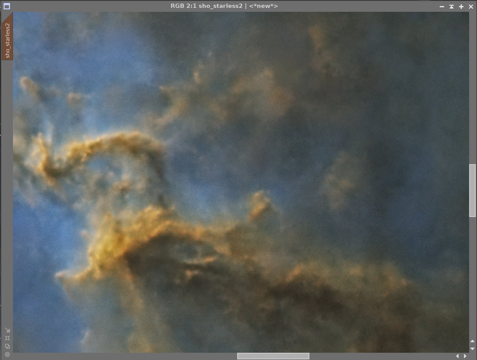
SHOStarless Image before LStarless Image is inserted
13. Insert L_Starless image options and choose the best
Use LRGBCombination to fold in Option #1 L-Starless Image - Aggressive Detail enhancement
Use LRGBCombination to fold in Option #2 L-Starless Image - Selective Detail enhancement
The aggressive one has a very blotchy background, and the sharp structures do not look natural. The Selective Detail Enhancement Approach wins the day!
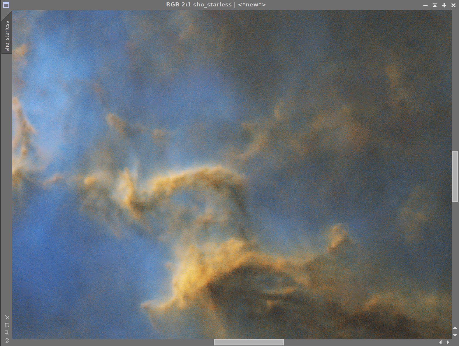
SHO_Starless with L-Starless (Aggressive) folded in (click to enlarge)
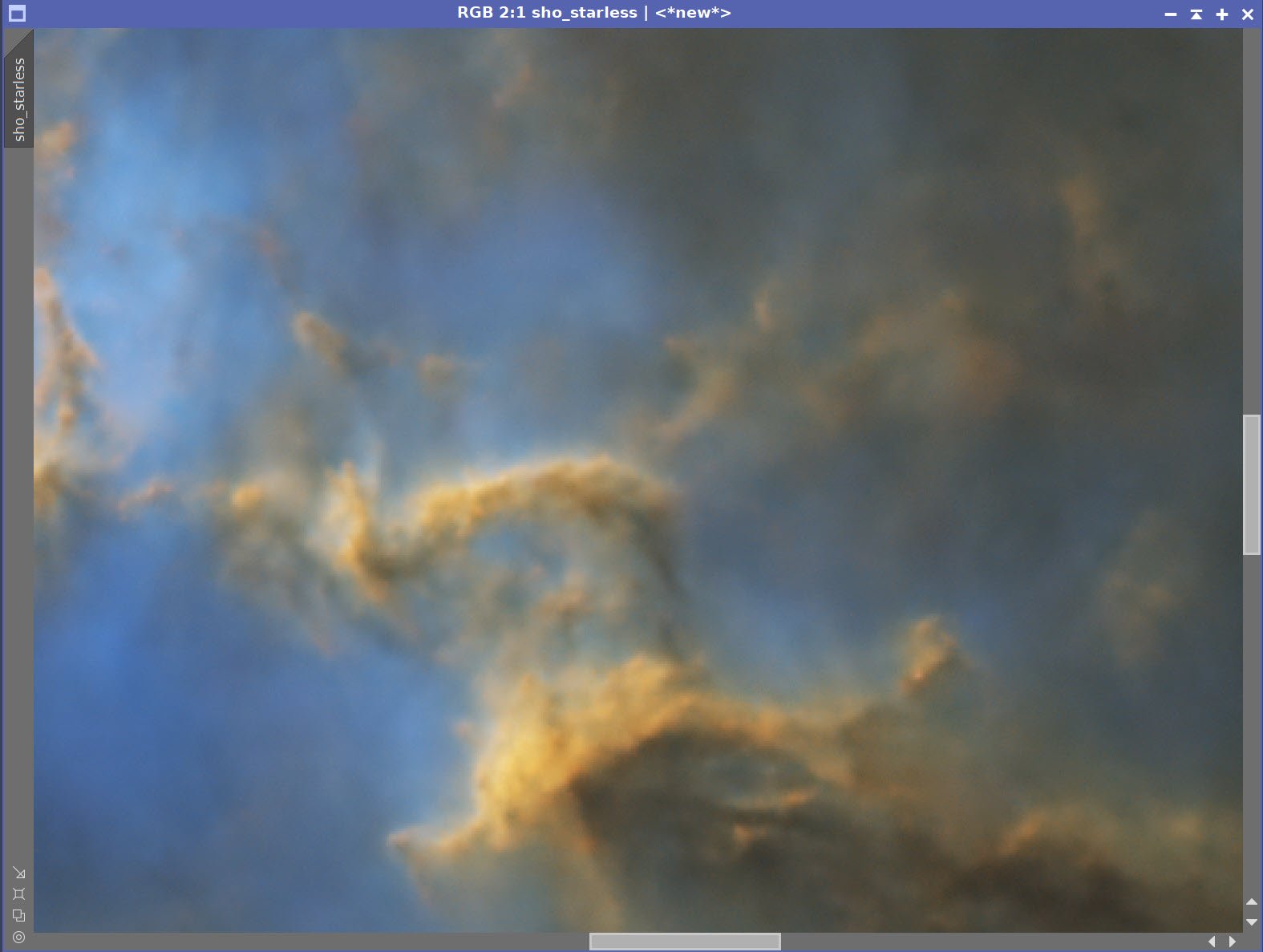
SHO_Starless wth L-Starless Opton #2 (Selective) folded in (click to enlarge)
14. Finish Processing the SHO_Stareless Image
Apply the Lum Mask and Invert
Apply Noise XTerminaor 0.6
Invert the Lum Mask
Apply MLT Sharpening (same parameters as used before)
Apply a final CT

Apply CT and touch up tone scale and color.
Lum Mask (for sharpening) (click to enlarge)
Lum Mask Inverted (for Noise XT) (click to enlarge)

Before and After Noise XT, and Sharpening - All using the Lum Mask

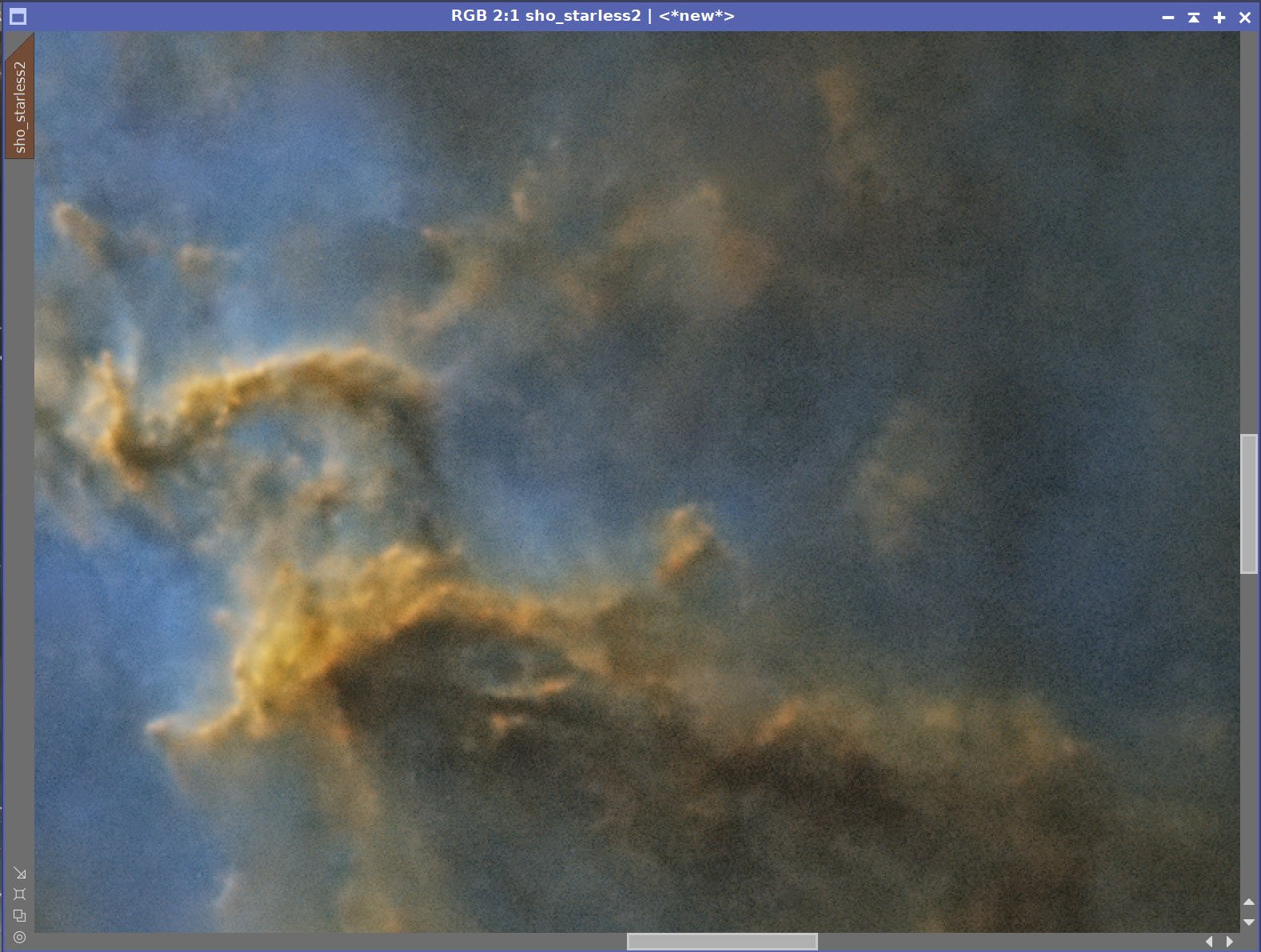
Final Starless Version After a final CT
15. Process the Stars-Only Image
I decided to use the SHOstarsOnly version of the stars so I could get some color in the stars- even if the color levels were very modest.
I used the CT to reduce the size of the stars and reduce the sat of the star colors
The Original SHO Stars-Only image (click to enlarge)
After Adjustment with CT (click to enlarge)
16. Add Stars Back In and Process
Using a screening equation and PixelMath, add the stars back in. See the PixelMath Panel snap below.

The PixelMath Script used to screen the stars back in.

Stars screened in.
17. Final Processing Touches
I’d like to sharpen up the detail around the outside of the image
Create GAME Script that covers
Apply the mask and do LHE 64, 2, 0.18, 8-bit historgram
Run the DarkStructuresEnhance Script
GAME Mask covering outer detail (click to enlarge)
Showing what the GAME Mask is overing (click to enlarge)

After a light application of LHE with a targeting GAME mask applied.
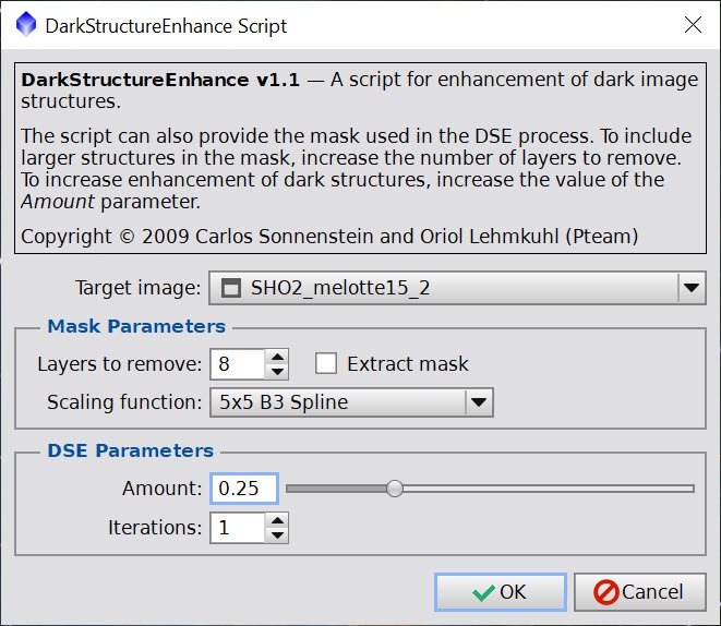
DarkStructureEnhance Parameters Used.

DarkStructuresEnhance.
19. Export to Photoshop
Save images as Tiff 16-bit unsigned and move to Photoshop
I tweaked things with the camera filter clarity, curves, and color mix - in a global adjustment
I used the lasso tool with a feather of 150 pixels and selected small areas of detail in the yellow region and enhanced them with the Clarity tool.
I added watermarks and title sections
Export Clear, Watermarked, and Web-sized jpegs.
The Final Image
I was very excited to get the ZWO ASI2600MM-Pro camera a while back. I ordered it when it was announced and then prepared to wait a long time to get it. When I did get it - I decided to put it onto the AP130 platform. That meant that I could move the ZWO ASI1600MM-Pro, along with its filter wheel over to my William Optics Platform. This now means that all of the platforms have been moved over to a mono camera and my ZWOASI924MC-Pro is now not in use.