
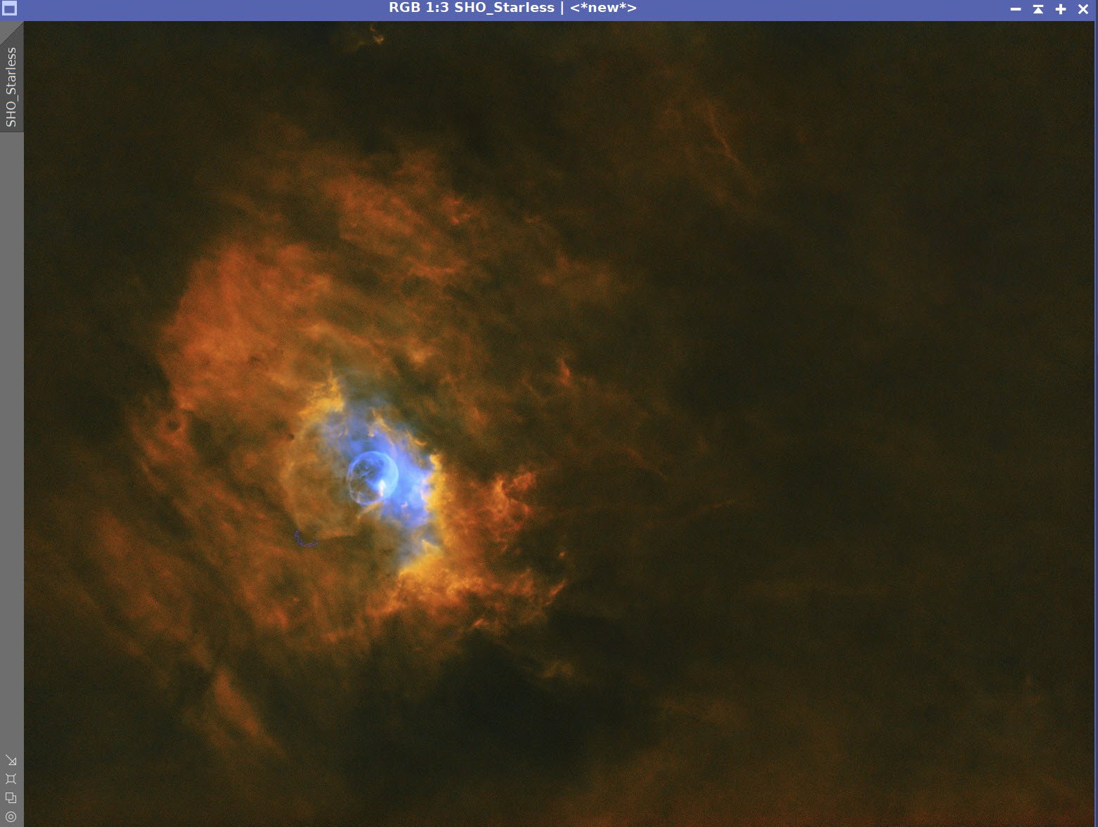
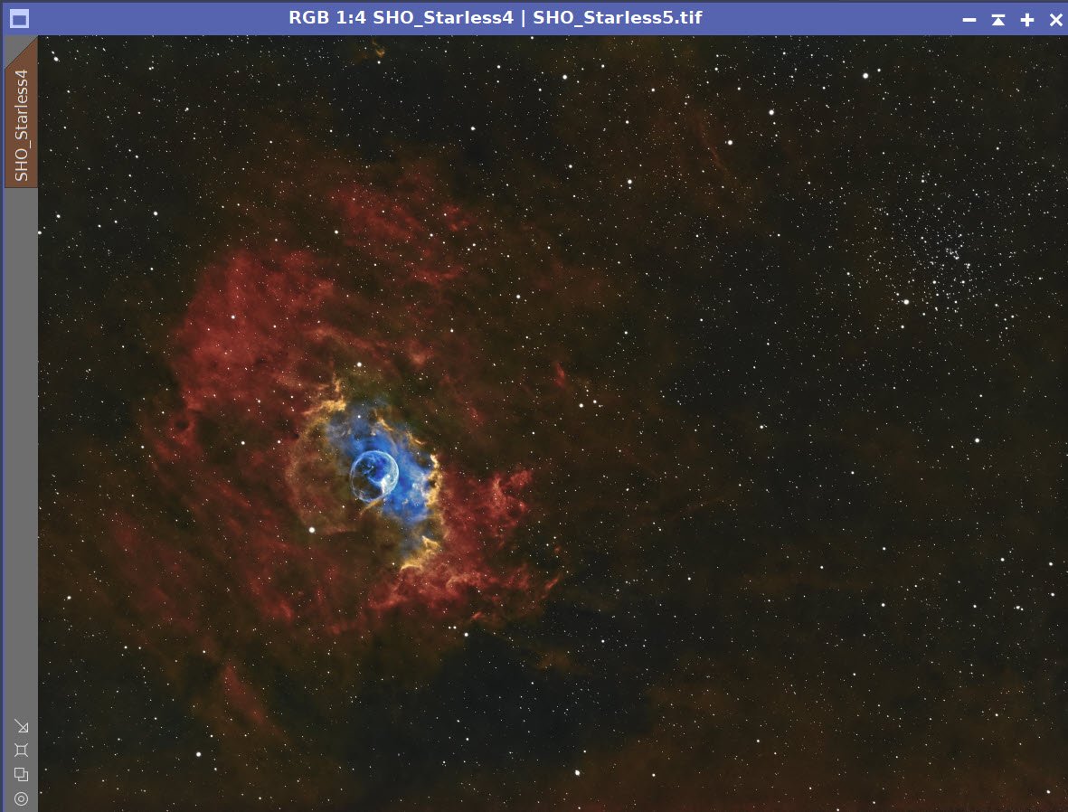
NGC 7635 - The Bubble Nebula w/M52 - 8.25 hours in SHO - Not Sure I Love it.
Date: Nov 12, 2022
Cosgrove’s Cosmos Catalog ➤#0114
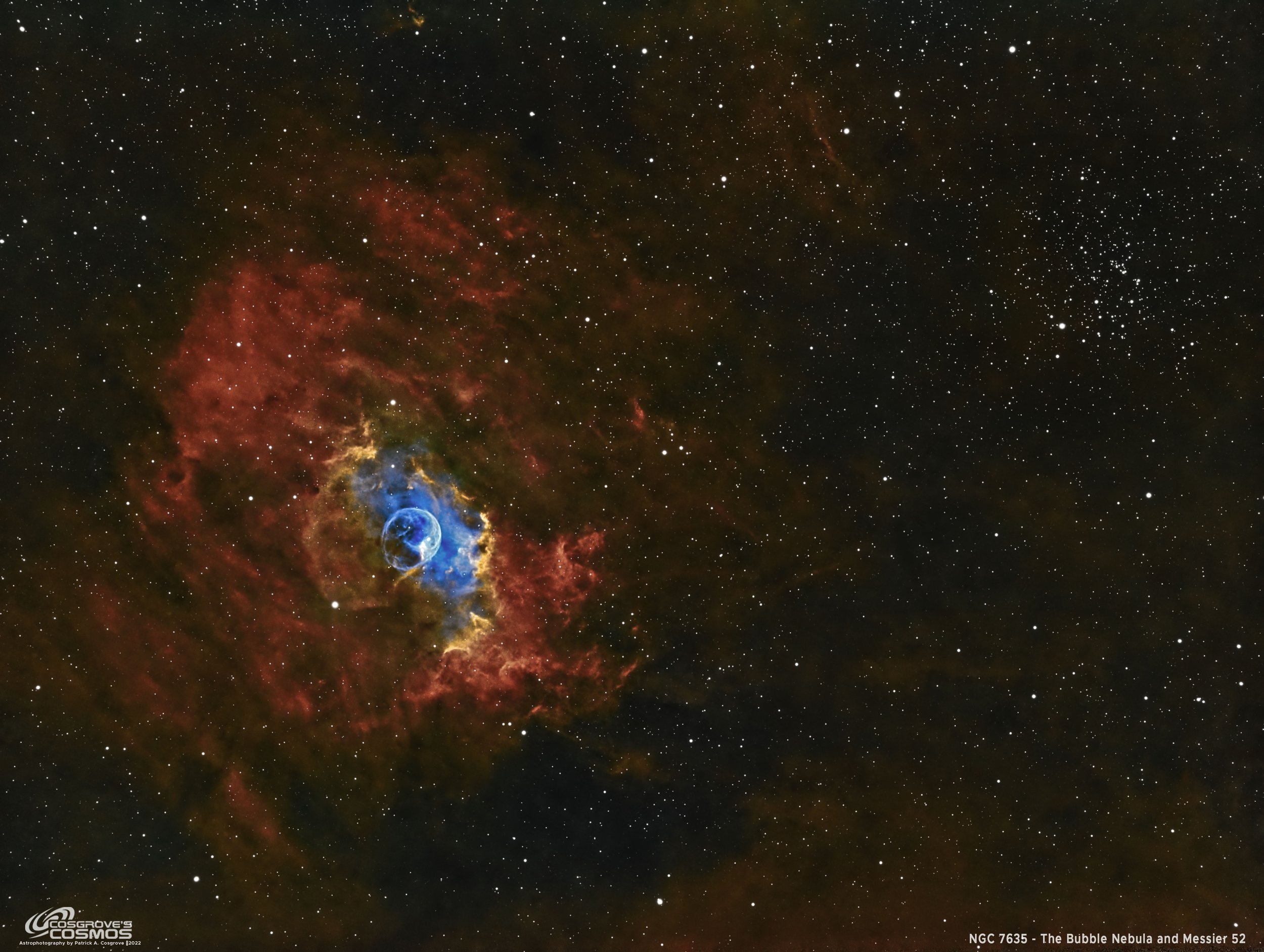
NGC 7635 - The Bubble Nebula with the Open Cluster Messier 52. (click for full res version via Astrobin.com)
Table of Contents Show (Click on lines to navigate)

Friedrich Wilhelm Herschel (1738-1822). Image taken from Wikipedia.
About the Target
NGC 7635 - The Bubble Nebula, also known as Sharpless 162 and Caldwell 11, is located between 7,100 and 11,000 light-years away in the constellation of Cassiopea.
This area is a rich HII region, and the “bubble” itself was created by stellar winds from a massive hot blue Wolf-Rayet star, AO 20575, that shed its material about 300,000 years ago to form the bubble. This star is 44 times larger than our sun. The Bubble itself is found in a massive molecular cloud that acts to contain the bubble's expansion and is excited by the same star, causing it to glow as well.
It was discovered in 1787 by William Herschel.
Messier 52, also known as NGC 7654, is an open cluster located in the same constellation located 4600 light-years away. It was discovered by Charles Messier in 1774.
Wikipedia tells us:

Charles Messier (1730-1817). Image Taken from Wikipedia
R. J. Trumpler classified the cluster appearance as II2r, indicating a rich cluster with little central concentration and a medium range in the brightness of the stars.[8] This was later revised to I2r, denoting a dense core.[6] The cluster has a core radius of 2.97 ± 0.46 ly (0.91 ± 0.14 pc) and a tidal radius of 42.7 ± 7.2 ly (13.1 ± 2.2 pc).[4] It has an estimated age of 158.5 million years[1] and a mass of 1,200 M☉.[4]
The magnitude 8.3 supergiant star BD +60°2532 is a probable member of the cluster,[4] so too 18 candidate slowly pulsating B stars, one being a Delta (δ) Scuti variable, and three candidate Gamma Doradus (γ Dor) variables.[9] There may also be three Be stars.[10] The core of the cluster shows a lack of interstellar matter, which may be due to supernovae explosion(s) early in the cluster's history.[6]
The Annotated Image

This annotated image was created using the Pixinsight ImageSolve and ImageAnnotation scripts.
The Location in the Sky

This finger chart was created in Pixinsight using the FinderChart process.
About the Project
Intro Video
A few minutes of introduction for this project by yours truly! While the processing walkthrough at the end of this post is quite detailed, sometimes it is hard to determine why some steps are done in the sequence they are. I wanted to find a way to have a 50,000-foot view and get a sense of the forest versus the trees.
Happy with the Result?
Actually - I am not.
Some images practically process themselves - others come into the world kicking and screaming the whole way. This is one of those images.
I am not sure I like the result. While I am a “color” guy - this image has more contrast and saturation than I like. So - what’s the problem? Just reduce the sats and the contrast, and voila - Bob’s your Uncle! Right?
Well no.
I have done those things, and you know what? I dislike those images even more!
I cannot quite put my finger on what it is about this image that bothers me.
Ultimately I relied on input from trusted astrophotographers in the area, and I posted this on the Twitter #Astrophophotography world based on the input there, I did make some final changes.
But I am still not completely happy.
Maybe it is just this target. I feel that when I lighten things up, the Bubble nebula gets “muddy” looking.
Maybe it’s because I am just recovering from an illness that really threw me for a loop.
Maybe it’s because I’m becoming a cantankerous old fart, and I feel the need to be contrarian - even with myself.
At any rate, I am “done” with this image and moving on.
What do YOU think about this image? Good? Bad? Meh? Since I am so divided on this, I would appreciate hearing YOUR opinion to help calibrate my own.
Choosing the Target
This is the second target I have processed from my capture session in late October.
I was away from home for a few weeks with plans on returning home just in time to start the next capture cycle. With longer nights, I had planned on capturing two waves of targets for each scope - and I made my plan accordingly.
As I looked for what targets would be well positioned for me (and my tree line), I saw that the Bubble Nebula would be within reach from about 10 pm until about 2 am.
I had shot the Bubble Nebula before, but I was not super satisfied with my result. I thought this might be a good target to revisit. If I could get an integration that was substantially longer than my previous effort - that would be a great starting point. Hopefully, my processing skills have also evolved and, between the two, would get a superior result.
Such was my plan.
I decided to capture this on my William Optics 132mm platform. I used SGP’s Mosaic and Framing Wizard to get a nice composition that included the open cluster M52 in the field. I was all ready to go!
The first problem, of course, was the fact that I came home sick with a bad cold.
Cold? HA! “I laugh at you. You will not stop my photon collection efforts.”
Of course, the cold responded: “Oh yeah, old man? - try me - you try me…..”
So I worked through the cold. Staying up all night. Being out in the cool night air.
The cold evolved into something all-consuming. I was miserable - just miserable.
While I had the luxury of two additional clear nights - they did me no good because I was so sick that I did not care anymore. So I missed two perfectly good nights and ended up with half of the integration that I was aiming for!
I also decided that I had to start taking better care of myself these days. I am not 20 years old anymore. The targets will be there - regardless if I am there or not. I had better make more effort to ensure I am still around to be there! :-)
Data Capture
I captured subs over two nights: Oct 21 and 22.
In general, these nights were clear and cool. The first night was a bit breezy, and I was concerned about my guiding given that my scopes are in the driveway and exposed - but the guiding stats looked good, and the subs showed good star images. I did not think either night was particularly transparent - but my subs seem to be looking reasonable, and I was satisfied.
Data Analysis
Blink analysis showed that the data looked pretty good for all filters. I did have one frame that was full of a weird noise signal. I have seen this before with this particular camera and just removed that sub. No other subs needed to be removed.
I then did a SubFrameSelector analysis focusing on star size (FWHM) and eccentricity. When I have a lot of subs, I can be quite aggressive in eliminating the outliers for these parameters. But I only had two nights of data with 5-minute subs - so I knew going in that I could not be very aggressive about this at all, or I would impact my integration times. In this case, I just removed the worst of the worst. In the end, I only removed a total of 5 subs for problems here.
Basically - I ended up with a pretty solid data set.
Previous Efforts
This is the third time that I have imaged NGC 7635
The first time was in September 2020 - using the same basic scope and camera. This was a 6.25-hour narrowband integration. It can be seen HERE. At the time, I was pretty happy with it. To y eye now, it looks muddled.
My second attempt was really an attempt on the Lobster Claw. But since the Bubble Nebula was in the neighborhood, I composed things to have both objects in the same frame. This was shot in December 2021 and was a 4.25-hour narrowband integration taken with my widefield FRA400 rig. It can be seen HERE.
The Bubble Nebula in this image looks very similar to my first one, but the nebula was a bit more orange in color.
The latest one has a darker nebula (to show the bubble better) and is much redder. It looks very different.
But is it better? Good question!
Here are all three, side-by-side, for comparison:
2020 (click to enlarge)
2021 (click to enlarge)
2022 (click to enlarge)
Image Processing
The image processing was pretty straightforward and follows a basic workflow that I find myself now using again and again when I am shooting narrowband SHO images.
I created a synthetic luminance image by using ImageIntegraton to combine the Ha, O3, and S2 images.
I then shifted to a starless workflow, which gave me great control over the processing of the nebula. I used carefully crafted Red, Green, Blue, and Range masks to process the color of the nebula itself.
I processed the L image for detail and sharpness and the color image for low noise and good color.
Finally, I added the L image to the SHO image and screened in some reduced stars (from the L image),
I spent WAY TOO MUCH time playing around with color variations on this image because I was not happy with where I ended up. I did not document all of the positions tried - but I did capture some, and I will share them in the section processing walkthrough below.
Sometimes I need to step away from the computer and ask for input from others. I did this time, and I will document that as well.
Below is a chart that - from a high level - summarizes my process flow for this image.

A high-level diagram of my processing workflow
A detailed Processing Walk-Through is provided for this image at the end of the posting…
Capture Details
Lights Frames
Data were collected over two nights: Oct 21 & 22
Number of subs after Blink and removal
35 x 300 seconds, bin 1x1 @ -15C, Unity Gain, Astrodon 5nm Ha
34 x 300 seconds, bin 1x1 @ -15C, Unity Gain, Astrodon 5nm O3
30 x 300 seconds, bin 1x1 @ -15C, Unity Gain , Astronmiks 6nm S2
Total of 8.25 hours
Cal Frames
25 Darks at 300 seconds, bin 1x1, -15C, Unity gain
15 Flats at bin 1x1, -15C, Unity gain - for Ha, O3, & S2 filters
25 Dark Flats at Flat exposure times, bin 1x1, -15C, Unity gain
Software
Capture Software: PHD2 Guider, Sequence Generator Pro controller
Image Processing: Pixinsight, Photoshop - assisted by Coffee, extensive processing indecision and second-guessing, editor regret, and much swearing…..
Capture Hardware:
Scope: William Optics 132mm f/7 FLT APO Refractor
Focus Motor: Pegasus Astro Focus Cube 2
Cam Rotator: Pegasus Astro Falcon
Guide Scope: Sharpstar 61EDPHII
Guide Focus Motor: ZWO EAF
Mount: Ioptron CEM 60
Tripod: Ioptron Tri-Pier
Camera: ZWO ASI1600MM-Pro
Filter Wheel: ZWO EFW 1.2 5 x8
Filters: ZWO Gen II 1.25” LRGB,
Astrodon 5nm Ha & O3 filters,
Astronomiks 6nm S2 filer
Guide Camera: ZWO ASI290MM-Mini
Dew Strips: Dew-Not Heater strips for Main & Guide
Scopes
Power Dist: Pegasus Astro Pocket Powerbox
USB Dist: Startech 8 slot USB 3.0 Hub
Polar Align Cam: Polemaster
Software:
Capture Software: PHD2 Guider, Sequence Generator Pro controller
Image Processing: Pixinsight, Photoshop - assisted by Coffee, extensive processing indecision and second-guessing, editor regret, and much swearing…..
Click below to see the Telescope Platform version used for this image:
Image Processing Walk-Through
(All Processing is done in Pixinsight - with some final touches done in Photoshop)
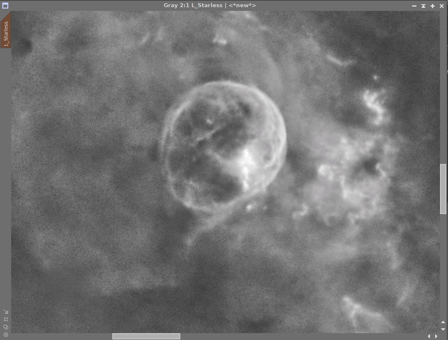
Weird noise sub that was removed. (click to enlarge)
1. Blink Screening Process
Ha
Nice clear signal
No trails or gradients
One frame was removed for a weird noise image
O3
Good
No trails
Some slight gradients
No subs removed
S2
all looks good
None removed
Flats
All looked good except for one night of Ha flats that looked like darks - not sure what happened here, but these were removed.
Dark flats
Looks good
Darks
300-sec darks all looked good.
2. WBPP 2.5.0
Reset everything
Load all lights
Load all flats
Load all darks
Select - maximum quality
Set Keyword: Night
Reg reference - auto - the default
Select the output directory to wbpp folder
Enable CC for all light frames
Pedestal value - auto for NB filters
Darks -set exposure tolerance to 0
Lights - set exposure tolerance to 0
Disable integration mode - just cal and alignment
Map flats and darks across nights
Ran with no problems - 55 minutes
Executed in 26 minute - no errors

WBPP Calibration view.

WBPP Post-Calibration View

The new pipeline screen for WBPP version 2.5
3.0 Use SubFrameSelector to analyze the Calibrated subs
When I have deep integration and shorter exposure times, I typically use SubFrameSelector to analyze for str bloat (FWHM) and eccentricity (guide errors). I tend to be aggressive at eliminating frames that have significant issues in either area. This, I find, greatly helps sharpness.
However, in this case, I have longer 5-minute exposure times, and my integration is not deep. Frankly, I can’t afford to walk in and start throwing out subs aggressively. Instead, I use SubFrameSelector to get a better sense of the issues in my data and find those frames that have the very worst problems. I may eliminate them - or in other cases, I plan on using the rejection logic during the integration cycle to minimize the impact of these problematic frames.
Actions Taken from this analysis:
Ha: 2 subs removed for FWHM
O3: 2 subs removed - for ECC and FWHM
S2: 1 sub removed for ECC
Ha Sub FWHM - Note eliminated frames (click to enlarge)
O3 Sub FWHM - Note eliminated frames (click to enlarge)
S2 Sub FWHM - Note eliminated frames (click to enlarge)
Ha Sub Eccentricity - Note eliminated frames. (click to enlarge)
O3 Sub Eccentricity - Note eliminated frames (click to enlarge)
S2 Sub Eccentricity - Note eliminated frames (click to enlarge)
4. Create Master Linear Images
Run ImageIntegrtion for each filters. Note ImageIntegration setting used in the panel view below.

The ImageIntegration Panel showing settings used for each integration cycle.
Rejection High - Ha (click to enlarge)
Rejection Low - Ha (click to enlarge)
Rejection High - O3 (click to enlarge)
Rejection Low - O3 (click to enlarge)
Rejection High - S2 (click to enlarge)
Rejection Low - S2 (click to enlarge)
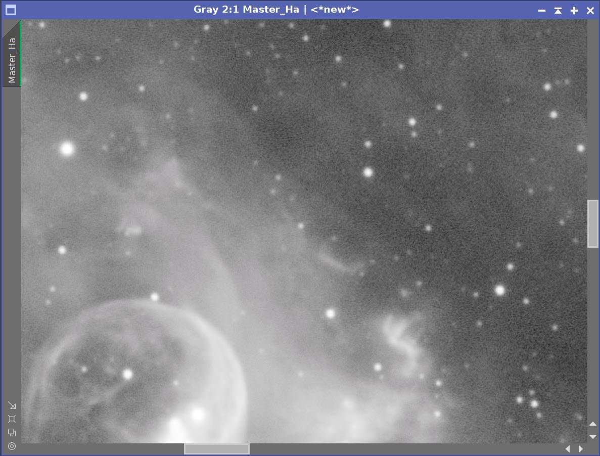
Master Ha (click to enlarge)
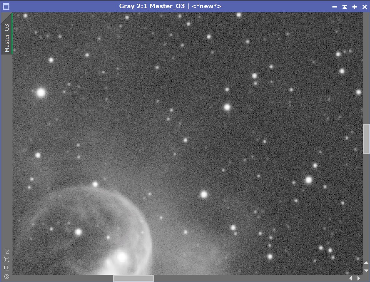
Master O3 (click to enlarge)
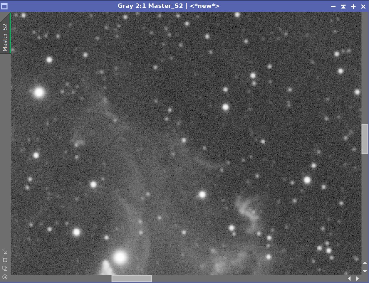
Master S2 (click to enlarge)
5. Crop all of the images
A common crop level was selected, and DynamicCrop was used to trim all of the master frames.
The edges were remarkably clean. Only a little had to be removed from the right edge.
6. Dynamic Background Extraction
DBE was run for each image using the subtraction method. Below are the Sampling plans, the before image, the after image, and the removed background images.
DBE: Ha Sampling (Click to enlarge)
Ha image Before DBE (click to enlarge)
Ha image After DBE (click to enlarge)
Ha background removed (click to enlarge)
DBE: O3 Image Sampling (Click to enlarge)
O3 Image Before DBE (click to enlarge)
O3 Image After DBE (click to enlarge)
O3 background removed (click to enlarge)
DBE: S2 Sampling (Click to enlarge)
S2 image Before DBE (click to enlarge)
S2 Image After DBE (click to enlarge)
S2 background removed (click to enlarge)
7. Apply light Noise Reduction to the Ha and O3 Linear Master Images
Apply Noise XTerminator with a value of 0.5.


Master Linear Images - Before and After Noise XTerminator 0.5
8. Create and Process the Synthetic Lum image
We only have three master images, which means we can use ImageIntegration to create the Synthetic Luminance Image.
Write the 3 master images to file.
Set up ImageIntegration to use those files, averaging for integration, and disable rejection.
Run and rename the new Luminance image.

ImageIntegration Panel as used to create the Synthetic Lum image.

The weights computed by ImageIntegration to combine the images

The computed Lum Image.

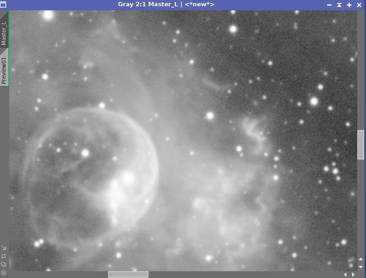
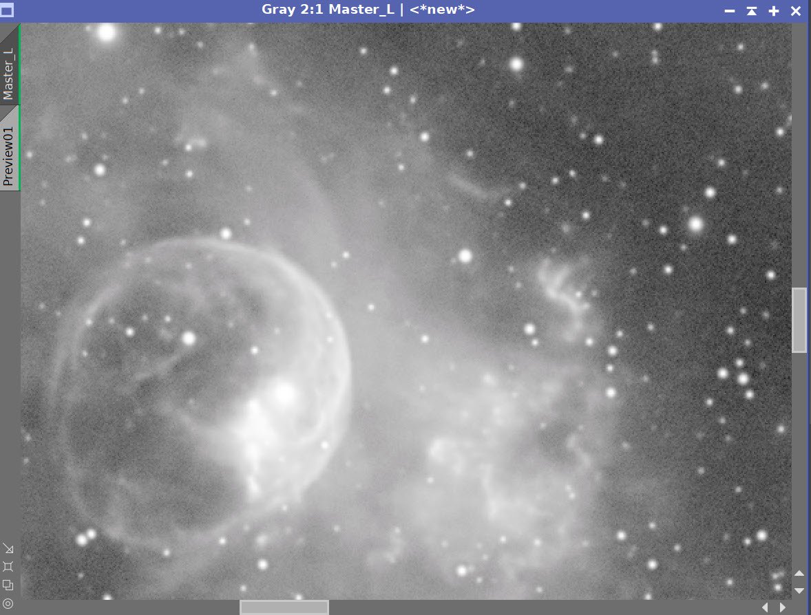
A 4-up panel showing the original and new computed L image for comparison.
9. Process the Linear Master L Image
Prep for Deconvolution
Run PsfImage and create the PSF file

The PFSImage Panel with settings used

The final PSF image
Run Starmask to create the initial LDSI image (see panel snap for parameters)

The StarMask panel set up to create the LDSI map.

The HT tool was used in this config to boost the LDSI image
Compare the mask to the original image - the stars are too small.
Apply HT Boost ( see panel snap for parameters) 2 or more times until star sizes match.

The Final LDSI image
Select Preview regions on the image for Decon exploration

These preview regions were selected to iteratively test the decon panel parameters for optimized results.
Iteratively run decon on previews until parameters are finalized (see panels snap for final values)

The final Deconvolution Parameters are shown
Master L - Before and After Deconvolution
Take the Lum image nonlinear using the STF->HT method. I am not worried about star growth as I will be doing starless processing.

The initial nonlinear L image.
Create a Starless Version of the image using Str Exterminator - creating a star image as well as using “Unscreen Stars”

The RC-Astro StarXTerminator Panel with settings used.
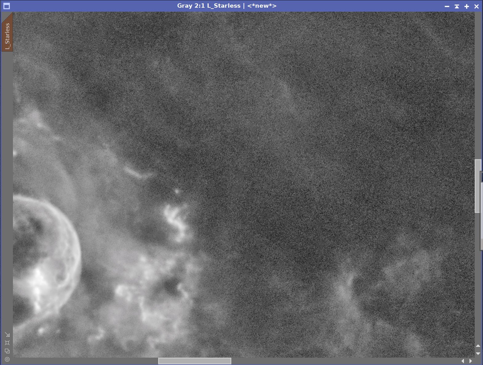
The Initial Starless L image (click to enlarge)
The initial Stars-Only Image (click to enlarge)
Enhance detail of the using Local Histogram Equalization
Enhance small-scale detail with LHE rdius=64, contrast limit=2, Amount=0.18, and 8-bit histograms
Enhance larger-scale detail with LHE rdius=244, contrast limit=2, Amount=0.25, and 10-bit histograms
Small-Scale LHE enhancement (click to enlarge)
Larger-Scale LHE enhancement (click to enlarge)
Create a range mask to isolate the bright region around the Bubble.
Apply the range mask and Invert it. We are now addressing the darker regions. Apply Noise XTerminator with a value of 0.6.
Invert the mask again - now we are focused on the area of the bubble.
Apply MLT sharpening
The range mask created. (click to enlarge)
The range mask targeting surrounding areas for NR (click to enlarge)

The range mask targeting central areas for Sharpening (click to enlarge)

The MLT panel with the sharpening parameters used.

Masked Regions - Before & After Noise Reduction and Sharpening
Final Starless Lum Image.
10. Create the Color SHO Image and Process
Take the Ha, O3, and S2 images nonlinear using the STF->HT process.
Review the three images and adjust using CT so they compare better one to another.

The original nonlinear images: Ha, O3, and S2.

After hand-tweaking the images.
Create the initial SHO color image using the ChannelCombination Tool.
Remove excess Green with XCNR
Invert the image. Magenta Areas are now green. Remove the “Green” bias with XCNR
Invert the image.
Adjust for tone scale with CT
Adjust color with ColorSatruation tool
The initial SHO color image. (click to enlarge)
Invert the image. Now magenta areas are green (click to enlarge)
After XCNR for Green. (Click to enlarge)
Apply XCNR for green. (click to enlarge)

Invert the image and adjust globally with CT.
Selective color adjustment with the ColorSaturation Tool (click to enlarge)

The curve used in the ColorSat tool .
Create a Starless version of the image using Star XTerminator
Create Color Masks with the ColorMask Script, dropping 2 layers for softness
Red
Green
Blue
Apply the Green Mask and adjust CT
Apply the Red Mask and adjust CT
Apply the Blue Mask and adjust CT
Remove masks and do an aggressive Noise XTerminator run with a value of 0.7
Fold in the L image using LRGBCombination
Adjust with CT

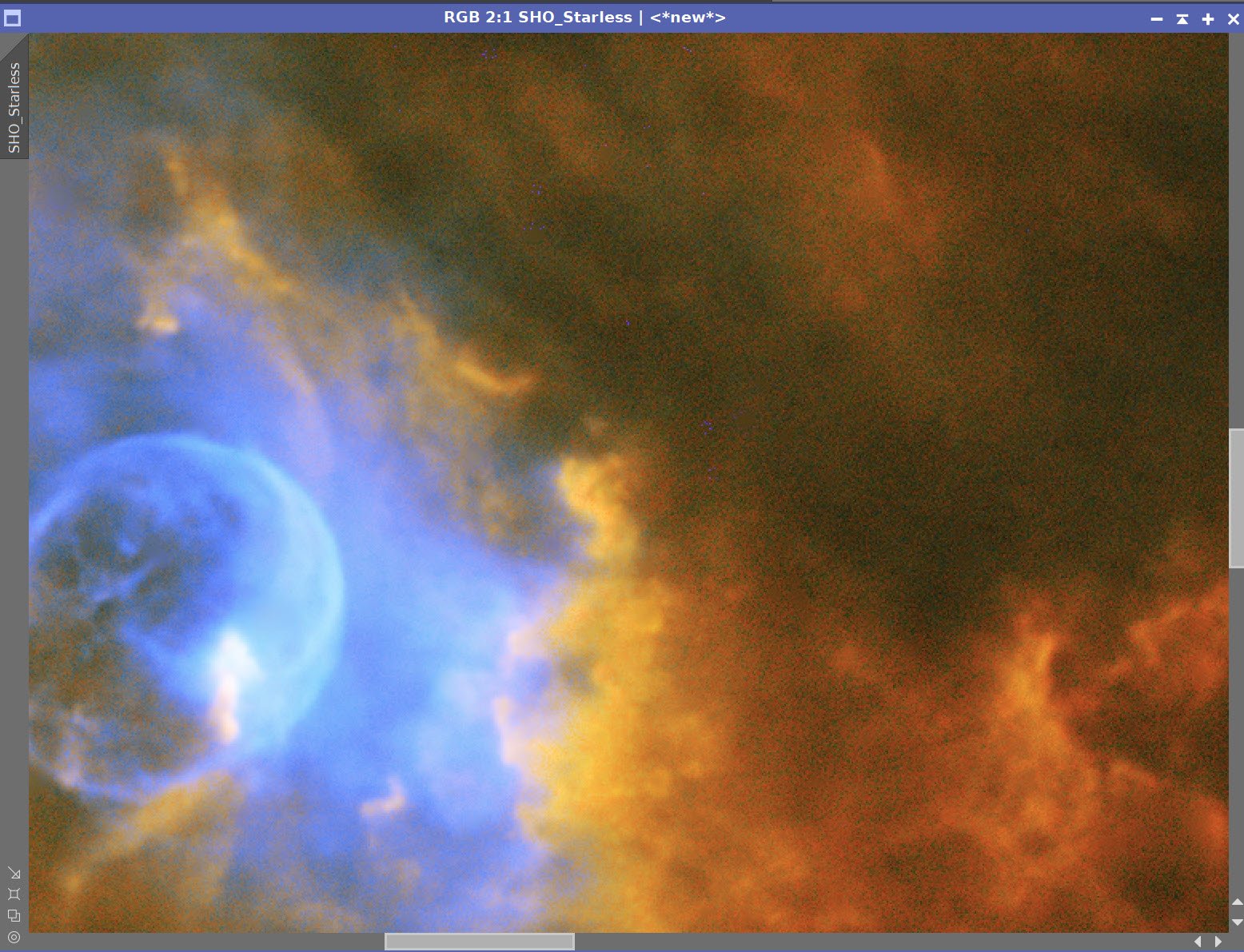
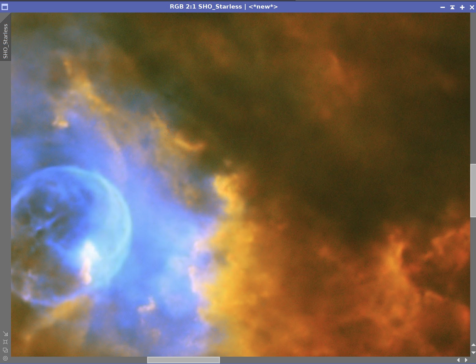
Initial SHO Starless image.
Red Color Mask (click to enlarge)
Green Color Mask (click to enlarge)
Blue Color Mask. (click to enlarge)

CT Green

CT Red mask
CT Blue
Before and After Noise XTerminator 0.7
After the Lum image was Inserted with LRGBCombination (click to enlarge)
After a CT adjustment. (click to enlarge)
11. Process the Stars-Only Image
Use the CT tool to reduce the intent and size of stars in the stars-only image.
The Original L Stars-Only image (click to enlarge)
After Adjustment with CT (click to enlarge)
12. Add Stars Back In and Process
Using a screening equation and PixelMath, add the stars back in. See the PixelMath Panel snap below.

The PixelMath Script used to screen the stars back in.

Stars screened in.

CT adjust to darken the background sky. (click to enlarge)

Creating a GAME Mask to to loosely isolate Bubble area
Invert GAME Mask and Adjust with CT (click to enlarge)
Invert the GAME mask again and adjust the center with CT. Use this as High color version. (Click to enlarge)
Use CT to create a Lower color version. (click to enlarge)
12. Assess Color Version
At this point, I had a high-color version and a second version that had more of a mid-color position with lower contrast. I was not happy with either. I experimented with different color positions, and I was not happy with what I was seeing.
If I went more yellow - trying to get the golden tones often associated with the Hubble Palette, things looked muddy to me.
If I tried to lighten the image, it also looked muddy to me.
I was not happy with this position, and I asked for some outside perspectives:
I asked two local astrophotography colleagues of mine, Dan Kutcha and Gary Optiz - I always respect the feedback these guys provide
I also shared the two images on Twitter #Astrophtography and asked for Feedback:
NGC 7635 - The Bubble Nebula - 8 hrs SHO.
— 🔭Cosgrove's Cosmos💫 (@CosgrovesCosmos) November 9, 2022
Having a hard time dialing in the color I want for this. It seems to want to be high in color and high in contrast. I can back off a bit, but it loses some snap.
So high color, mid color, or back off even more?#Astrophotography pic.twitter.com/HPHDcFQCa8
The feedback I got could best be summarized as this:
The slightly lower saturation position was preferred
The orange color looked odd - move back to a more a red color balance
Darken the red nebula to make the bubble stand out more and “pop”
Keep the blue color sat high
13. Finalize the Image
Make the desired changes
Adjust the star size
After moving the color balance more towards red. (click to enlarge)
Darken the red nebula with CT (click to enlarge)
Apply Bill Blanshan’s Star Reduction PM Script - V2 with a value of 0.35.
19. Export to Photoshop
Save images as Tiff 16-bit unsigned and move to Photoshop
I tweaked things with the camera filter clarity and curves
I used the lasso tool with a feather of 150 pixels and selected small areas of detail in the yellow region around the bubble, and enhance it with the Clarity tool.
Add watermarks and title sections
Export Clear, Watermarked, and Web-sized jpegs.

The Final Image
I was very excited to get the ZWO ASI2600MM-Pro camera a while back. I ordered it when it was announced and then prepared to wait a long time to get it. When I did get it - I decided to put it onto the AP130 platform. That meant that I could move the ZWO ASI1600MM-Pro, along with its filter wheel over to my William Optics Platform. This now means that all of the platforms have been moved over to a mono camera and my ZWOASI924MC-Pro is now not in use.