
SH2-157 The Lobster Claw Nebula - with NGC 7635 (The Bubble Nebula) in SHO - 4.25 hours.
Date: December 30, 2021
Cosgrove’s Cosmos Catalog ➤#0092
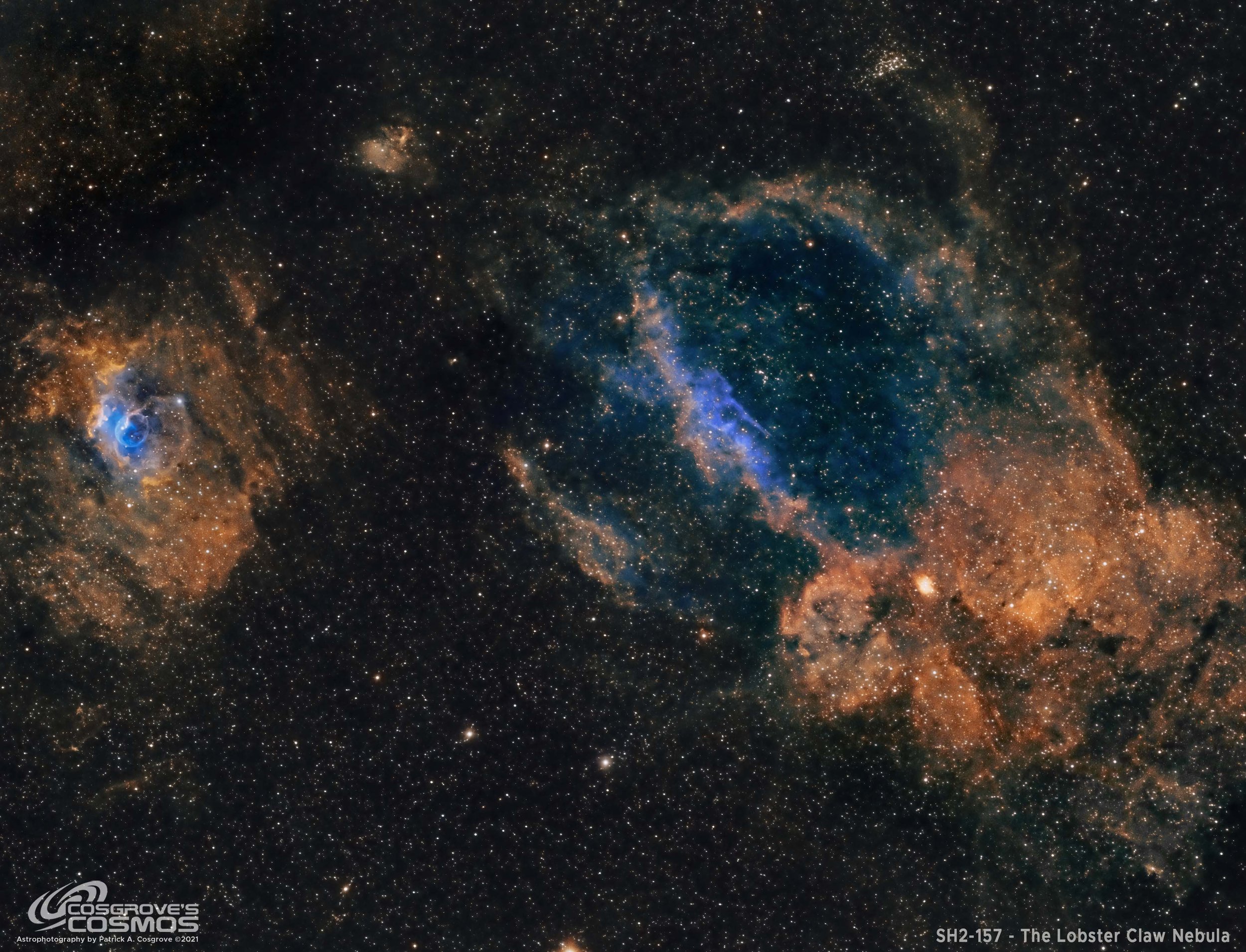
SH2-157 - The Lobster Claw Nebula - along with NGC 7635 (The bubble Nebula) visible on the left side of the field. (Click for high res version via Astrobin.com)
Table of Contents Show (Click on lines to navigate)
A Special Note:
The data collected on this project was reprocessed in Feb 2024 using new methods and new tools - resulting in an improved image. The posting for that more recent effort can be seen HERE.
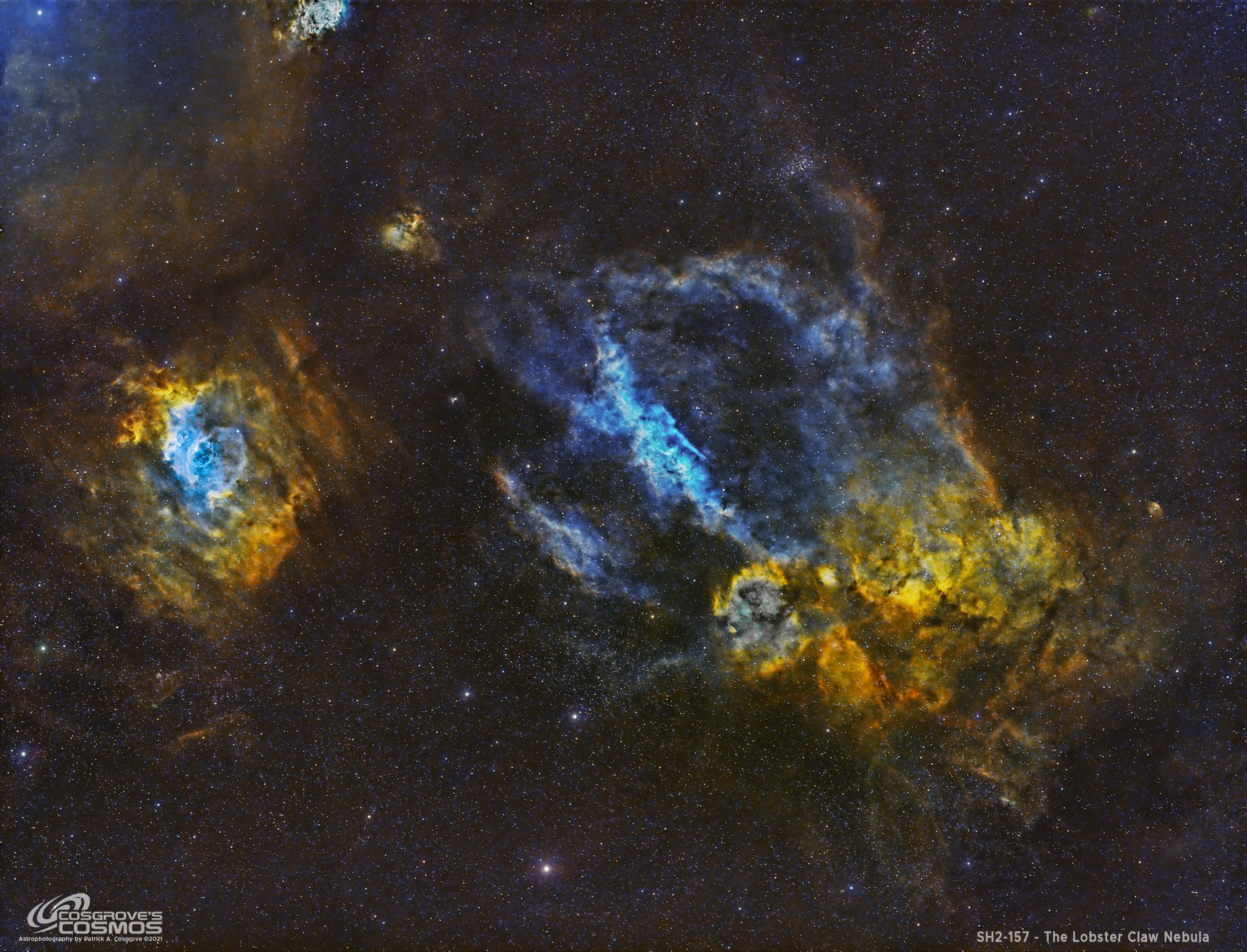
The reprocessed and improved image. (click to go to the newer post)
About the Target
SH2-157, also known as the Lobster Claw Nebula, is an emission nebula located about 11,000 light-years away in the constellation of Cassiopeia. The red/orange portions of the nebula are made up of strong HII regions. The predominantly yellow part of the nebula is a very large H II region. The blue-colored regions are predominately from the emission of light from molecular oxygen.
To the left of the image, you can see NGC 7635 - the Bubble Nebula, which is much more widely known. Also visible is the star cluster NGC 7510, seen at the top right of the image.
Annotated Image

Location in the Sky

This chart was created with the new Pixinsight FindingChart Process. This Image of the Lobster Claw Nebula is show in the red region above.
About the Project
The Lobster Claw Nebula is not as well known as many Astro targets - but I have seen some really nice images of it before and because of its unusual nature, I had added it to my target wish list. I thought I had my chance to grab it on November 8th this year. Many of my recent projects have come from a spate of wonderful clear skies with no moon that happened from Nov 5th through Nov 8th. With almost 12 hours of darkness, I shot as much as I could! On November 8th, I decided to try for a few new targets. I had heard that the clear weather that we had been having was due to continue for 2-3 more nights. As a result of this, I started a few new targets on the 8th and planned on continuing as long as the weather held out.
Well - the weather did NOT hold out and the 8th turned out to be the end of the clear skies!
As a result of this, I ended up with a few projects that were a little - shall we say - “lean” on integration time. The last project I published, IC 1848, was in the same boat. SO I have been processing these and seeing what I could do with the data.
On one hand, I must say that the resulting images are much better than I expected given the short integration times. On the other hand, I must admit that these are not examples of excellent results that I would like to show. So for now - these projects will show what can be done with shorter than optimal total exposure times. They are also a placeholder. One day I hope to get back to these images and add more data to them. Then perhaps I will have a new version that I can be unashamed of!
This image was shot with my Askar FRA400 Platform, which has a focal length of 400mm and an f-ratio of 5.5. This rig sports an ASI1600MM-Pro mono camera and I shot 300-second subframes using Ha. O3, and S2 narrowband filters.
The lower focal length of this rig allowed me to capture the entire area of the Lobster Claw while still having enough coverage to grab the Bubble Nebula.
Bubble Nebula Included!
I have shot the bubble nebula before with a rig with a much longer focal length. That project shows this interesting area of sky with far better details This project can be seen HERE.
A larger scale version of the Bubble Nebula shot last year. (click to enlarge)
A Critique of the Image
When I look at the individual Ha, O3 & S2 images, I see a very strong signal in the Ha image and very weak images on the O3 and S2 signals. This makes perfect sense - this is after all primarily an HII emission nebula. But the O3 and S2 images contribute important color information for the Hubble Palette SHO rendering. The relatively short exposure integration means that these layers are starved for photons and the resulting images are very noisy and not all smooth.
As a result of this, I had to be very aggressive with noise reduction. I did my normal Linear Noise reduction step using MLT, and a Nonlinear Nie reduction step using ACDNR using pretty aggressive terms. Finally, I used Topaz AI Denoise and Photoshop NR on certain spot areas.
When looking at the whole image - it came out reasonably well. However, if you do a deep dive and look at the image at the pixel level you can see some mottling in the background sky and some distortion around small stars. These would not likely happen if I had a lot more integration time.
Also, the orange color of the main part of the “Claw” lacks some variation in color that I think. would have had if the O3 and S2 images had more integration time on them.
So my final verdict? Not bad for a relatively short exposure on a faint object - but far from a great image. I will of course save all of my raw data and I hope to someday collect more data and create a better version of this image.
Fixing My Short Integration Time Problem
There are two primary drivers that cause me to end up with shorter than desired integration times: Cloudy skies and Trees!
In update New York, we end up having a lot of weather-driven by the Great Lakes. This means too many cloudy days and there is not a lot I can do about that. When we do have a clear moonless night, I do run 3 telescope platforms so that I can capture photons in parallel. I am planning on adding a fourth platform but this takes me only so far.
The other problem is TREES! My property has too many of them and they act to hem in the sky that I can see. To shoot a target, I have to wait for it to first clear the trees on the east side of the property and then I can shoot until the target hits the trees on the west side of the property. The time on target between these events is typically around 3 hours. This is way too limiting for a serious astrophotographer.
But this is one that I can do something about!
Are the chain saws coming out? Nope. But I have been retired for two years and my wife just retired this past summer. We have decided to move to a new home. We are currently searching to buy a property that is likely located to the south of our current location (darker skies) and we are looking for property sized between 3 and 20 acres that we could build a new house on - and more importantly - build a 15’x15’ Roll-Off-Roof Observatory with four piers! I am looking for open dark skies for the observatory and a section of trees for the house.
Since we are likely to build a new house, I am looking for an Architect that can design the house and create a stamped set of plans for the observatory. I am also looking for a custom builder that could build the observatory at the same time as the house.
Hopefully, within the next year or two, I will solve my “Tree” problem!
I will probably open a new section on this website as I begin to make progress on the observatory. Stay tuned!
Capture Details
Lights
Taken on the night of Nov 8th, 2021
20 x 300 seconds, bin 1x1 @ -15C, unity gain, Astronomiks 6nm Ha filter
16 x 300 seconds, bin 1x1 @ -15C, unity gain, Astronomiks 6nm O3 filter
15 x 300 seconds, bin 1x1 @ -15C, unity gain, Astronomiks 6nm S2 filter
Total of 4 hours 15 minutes
Cal Frames
25 Darks at 300 seconds, bin 1x1, -15C, gain unity
25 Dark Flats at each Flat exposure times, bin 1x1, -15C, gain unity
15 Ha, O3, and S2 flats
Capture Hardware:
Scope: Astrophysics 130mm Starfire F/8.35 APO refractorGuide Scope: Televue 76mm DoubletCamera: ZWO AS2600mm-pro with ZWO 7x36 Filter wheel with ZWO LRGB filter set,and Astronomiks 6nm Narrowband filter setGuide Camera: ZWO ASI290MiniFocus Motor: Pegasus Astro Focus Cube 2Camera Rotator: Pegasus Astro FalconMount: Ioptron CEM60Polar Alignment: Polemaster camera
Software:
Capture Software: PHD2 Guider, Sequence Generator Pro controller
Image Processing: Pixinsight, Photoshop - assisted by Coffee, extensive processing indecision and second-guessing, editor regret and much swearing…..
Click below to see the Telescope Platform version used for this image
Image Processing Detail (Note this is all mostly based on Pixinsight)
1. Assess all captures with Blink
Light images
All images look great - no gradients or problems seen
Flat Frames - no problems seen
Flat Darks
Taken from the IC1805 project. Greens are missing, but have the same exposure time as red so that we can use those.
Darks - taken from IC1805 project
2. WBPP Script
All images loaded into WBPP
Cosmetic correction enabled
Drizzle integration was chosen to deal with slight undersampling
Pedestal image of 50 used on Ha channel
Integration was enabled and this seems to simplify the DrizzleIntegration process for me.

The WBPP Preprocess Screen
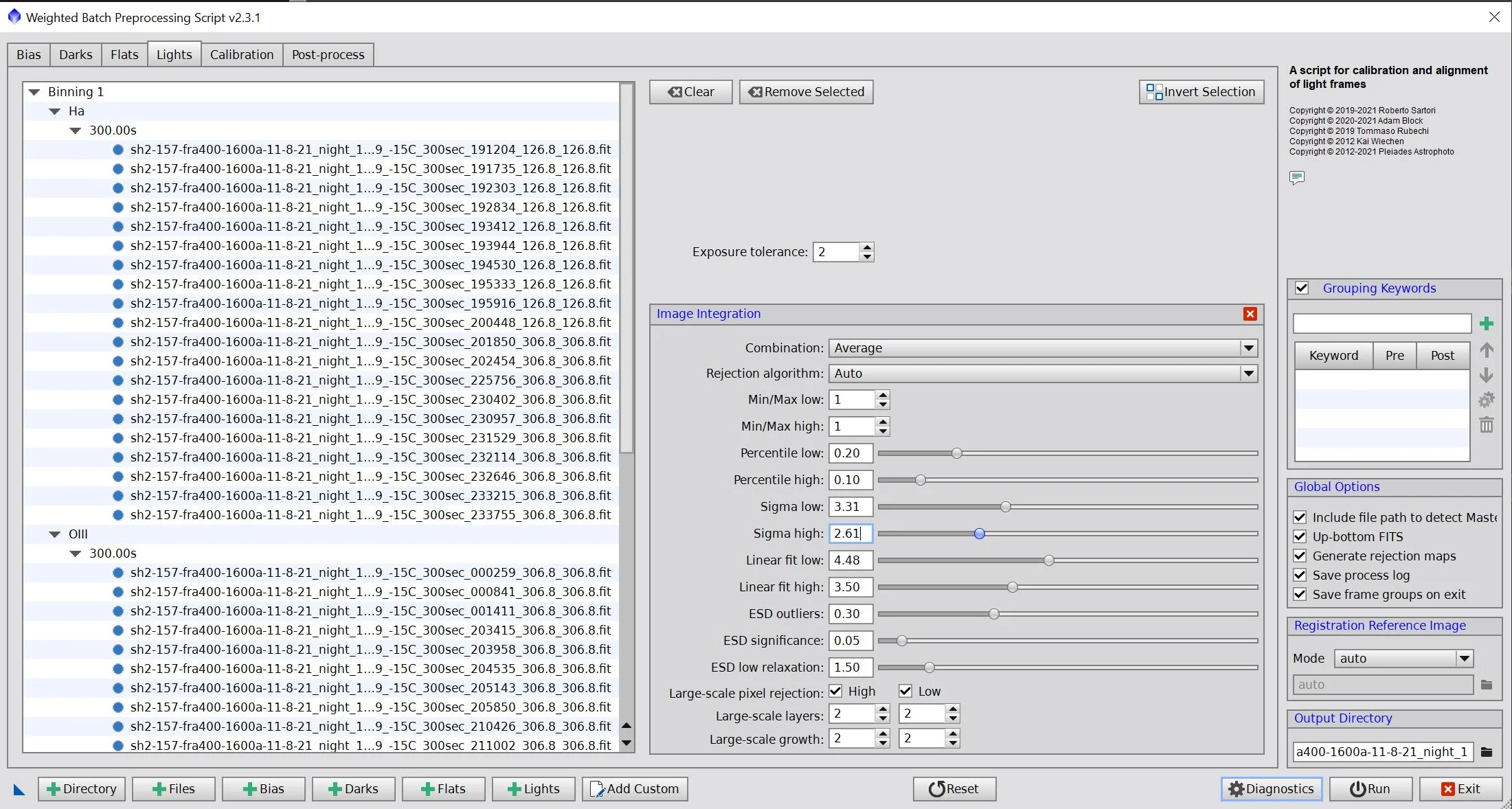
The Integration Screen showing rejection thresholds used.

3. DrizzleIntegration
Default paramters used
Run for each image to create all image masters.
4. Dynamic Crop
A common best crop position was used and implemented with DynamicCrop
5. DBE - no obvious gradients seen, so DBE was not run at this stage
6. Prep for Deconvolution
Object Masks were created for each layer.
A copy was made of the Linear images. Use STF->HT methods of creating a nonlinear image.
HT was used to adjust the mask so that the background sky was black, and most Nebula areas were white. Convolution run on mask 2X, with std dev = 4.
Create a local Support Image.
These are basically star maps of the biggest and brightest stars. Since these are usually saturated and clipped, they never have normal point spread functions, so they don’t fit the deconvolution model, and it does bad things to them. I probably only need to create one of these and use it for all images, but I tend to do a custom one for each color. Probably no real value in doing this.
This was created using the Ha image and used for all. I used Starmap with six layers and everything else set to default for this.
The final image was boosted a bit using HT
Psf files created- These are point spread function files. I created it using the PSImage Script. Piece of cake! See an example of what this tool looks like in use below.

The Ha Object Mask (click to enlarge)
The O3 Object Mask (click to enlarge)
The S2 Object Mask (click to enlarge)
The Ha Local Support Image (click to enlarge)
The O3 Local Support Image (click to enlarge)
The S2 Local Support Image (click to enlarge)

The Ha PSF image

The O3 PSF image

The S2 PSF image
7. Run Deconvolution
Set up several preview areas to test on each image
Apply the object mask
Set the deconvolution tool to use the right psf and local support maps
For each layer - explore what global dark value gives the best response without dark rings.
Ha: 0.008 20 interactions
O3: 0.02, 20 interactions
S2: 0.05, 20 interactions
The Ha Image before Deconvolution applied (click to enlarge)
The O3 Image before Deconvolution applied (click to enlarge)
The S2 Image before Deconvolution applied (click to enlarge)
The Ha Image after Deconvolution applied (click to enlarge)
The O3 Image after Deconvolution applied (click to enlarge)
The S2 Image after Deconvolution applied (click to enlarge)
8. Linear noise reduction
Apply MLT with the following parameters shown below
Test on preview and apply to each image.


The Ha image before the Linear Denoise Operation with MLT.

The O3 image before the Linear Denoise Operation with MLT.

The S2 image before the Linear Denoise Operation with MLT.

The Ha image after the Linear Denoise Operation with MLT.

The O3 image after the Linear Denoise Operation with MLT.

The S2 image after the Linear Denoise Operation with MLT.
9. Go Nonlinear and Combine Images
Now I am ready to go nonlinear. For each image:
Select a preview of the background sky
Use MaskedStretch with the selected preview to stretch the image
Balance the images with LinFit, using the Ha image as the reference image. This balances out the signals and background.
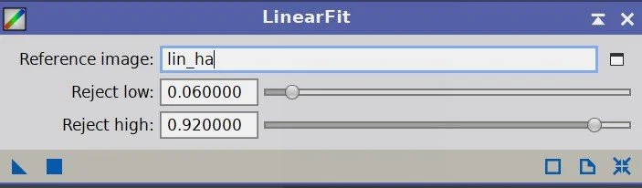
The Linfit panel as used. Note that the reject low is a bit higher and the reject high is a bit lower.

The balanced Nonlinear Images.
10. Create a Color SHO Image.
Use the ChannelCombination tool to create the initial SHO image. This image is very green - now remove the excess green.
SCNR with Green Channel
The problem now is the magenta stars in the region outside the nebula. Remove this by making a mask
Use the ColorMask script to select magenta - set blur layers to 1.
Now edit out the shape of the nebula and its interior from the mask using the DynamicPaintBrush.
Apply mask
Use CT to reduce the red curve
Initial SHO Image (click to enlarge)
Magenta Mask created with the ColorMask Script (click to enlarge)
ISHO Image after SCNR to remove green (click to enlarge)
The SHO image after the Magenta Mask was applied and CT used to reduce Sat (click to enlarge)
11. Apply DBE to remove some residual Color Gradients.
Pattern selected as shown below
Apply with subtraction.

DBE pattern to remove color gradients.
12. Create Color Masks and Enhance
Blue mask - use the ColorMask script with Blue chosen, 1 layer smoothing
Adjust mask
Use HT to boost
Run deconvolution on the mask to smooth it out
Green mask - ColorMask script with Green Chosen
Adjust the mask as in the blue example above
Apply Blue Mask
Adjust with CT - B layer and sat
Apply Green Mask
Adjust with CT R, G, B, and Sat
Run LHE Radius 64, Contrast 2.0, Amount 0.5, Histogram 8-bit
Run LHE Radius 200, Contrast 2.0, Amount 0.80, Histogram 12-bit
Using the GAME Script, create gradient masks for the bubble nebula and the claw regions of the image
Apply bubble and run HDRMT 8 layers
apply claw and use CT to adjust

Blue Mask

Game Mask for Claw Region

Green mask to adjust Orange regions.
Game Mask for Bubble Region

13. Apply Nonlinear Noise Reduction
Setup ACDNR Lightness Panel as shown
Setup ACDNR Chrominance panel as shown
Select several previews and test
Apply to the image.

ACDNR Lightness Panel settings

Before ACDNR Applied

ACDNR Chrominance

After ACDNR Applied
14. Tweak Star Colors
Create a star mask using StartNet
Boost with HT
Apply the mask
Use CT to adjust the star color
17. Star Reduction
Use the EZ-StarReduction script with the Adam Block method to reduce stars

Before EZ-StarReduction

After EZ-StarReduction
18. Move to PhotoShop
Export as 16-bit TIFF
Open in Photoshop
Use Camera Raw filter to tweak color, tone, and Clarity
Use Starshrink to reduce small stars
Use Starshrink to reduce large stars
Use Topaz AI Denoise to aggressively
Crop the image for better composition
Select regions of interest with the lasso and a feather of 150, and tweak usingthe Camera Raw filter.
Add watermarks
Export various versions of the image

The portable scope platform is supposed to be, well, portable. That means light and compact. In determining how to pack this platform for travel, I realized that the finder scope mounting rings made no sense in this application and I changed them out with something both more rigid and compact - the William Optics 50mm base-slide ring set.