
NGC 1499: A Narrow Field Shot of the - California Nebula - in SHO - 10 Hours
Date: January 5, 2022
Cosgrove’s Cosmos Catalog ➤#0093

A Zoomed in shot of the center of NGC 1499 - The California Nebula. (click for full res image via Astrobin.com)
Table of Contents Show (Click on lines to navigate)
About the Target
NGC 1499, also known as the California Nebula and SH2-220, is a large and faint emission nebula located about 1,000 light-years away in the constellation of Perseus. Notoriously difficult to see visually, NGC 1499 can easily be seen in long exposure images, measuring about 2.5 degrees on the long axis. The nebula's shape has been compared to the shape of the state of California, thus its name. This is a classic HII emission region, along with quantities of Sodium and very small amounts of molecular oxygen. The cloud system is probably illuminated by Xi Persei. This hot blue-white main-sequence star belongs to an association of young stars that probably arose from this interstellar cloud.
This nebula was discovered by E.E. Barnard in 1884, and it was added to Dreyer's NGC catalog shortly thereafter.
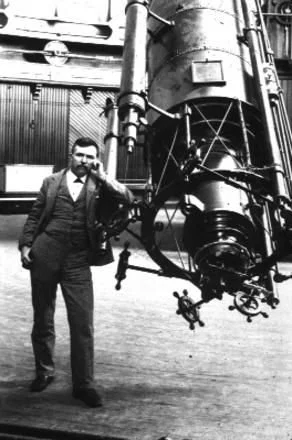
E.E. Barnard (December 16, 1857 – February 6, 1923)
The Annotated Image

The Location in the Sky

About the Project
November is typically a miserable month for astrophotography here in Western New York.
But not this November!
We had almost four clear moonless nights in a row - starting on November 5 and going through November 8th! The last night things began to deteriorate around 3 am, but since captures started around 7 pm, we had an opportunity for some good integration. Simply amazing!
This is the eighth image I have processed from that what was captured at that time.
This is also the FIRST image published in 2022! I recently built a powerful image-processing computer with a small form-factor case (ITX-Mini). I wanted something I could use traveling. I processed this image over the holidays while staying with my son and daughter-in-law. My wife and I were watching my little granddaughter, so all processing was done during nap times (hers - not mine!). This is my portable workstation from last week:
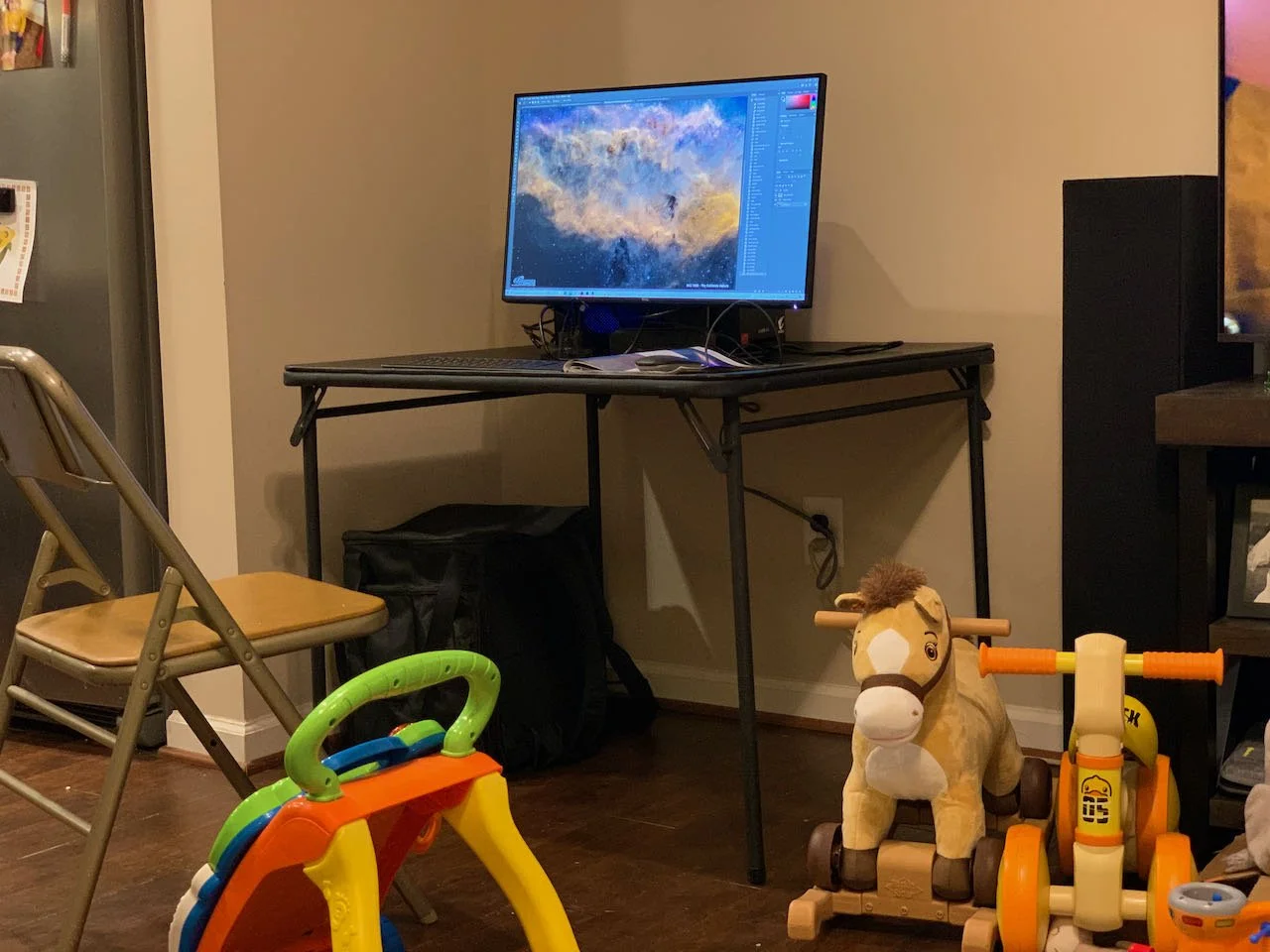
Note that during breaks, I had use of the pony and the bike! The downside was that the pony would sing “I am a little pony clippity-clop, clippity-clop” over and over until your ears began to bleed…..
Target Selection
With almost 12 hours of darkness and three scopes running at the same time - it was a bit of a challenge to create the shooting list for this data collection cycle. Complicating this is that each object had only about a three-hour window of availability because of the trees on my property. So I had to estimate the time slices to shoot what object on what telescope. This was easy as I started this process, but as I got down to fewer available cycles, it was tough to go find a suitable object that was a good match for the scope/camera combo that was available.
For one such block, the only thing that interested me was the California Nebula. Being a very large object, the Askar FRA400 would have been a better choice here - its 400mm focal length would have fit much more of the nebula in the frame. But was already allocated to another object at this time. What I did have available was the Astro-Physics 130mm scope with the ASI2600MM-Pro Camera. This scope has a focal length of 1080mm, so the only way to make this work was to pick an interesting part of the nebula and image it. I used the Framing and Mosaic Wizard in Sequence Generator Pro, and set up the composition. Here is the rough portion of the nebula targeted:
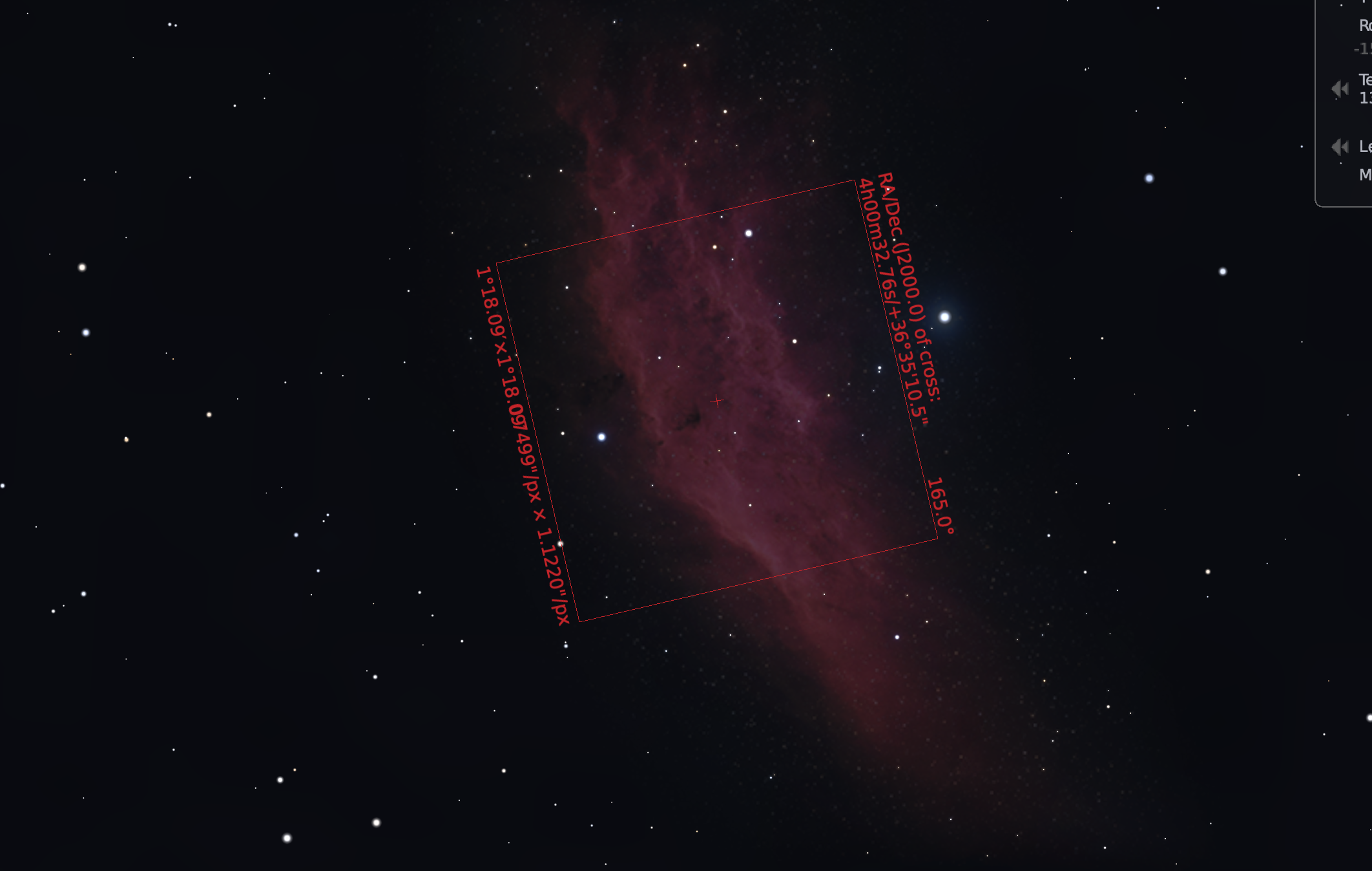
Image Capture
Subframes were captured over three evenings. Narrowband Ha, O3, and S2 subs were collected, resulting in 10 hours of integration. The Ha was the strongest signal, followed fairly closely by the S2 image, and then trailing in the distance was the O3 image. The O3 image was very faint - an indication that was little molecular oxygen in the nebula.
I ended up going with the lower-color version.
Image Critique
This image has a reasonable integration base with 10 hours - something I cannot do for all of my images either because of the weather or sky access limitations due to the trees on my property. But after 10 hours, the signal starts to clean up well. The Ha image and the S2 image have a solid signal, but the O3 single is very faint and requires more integration to bring this out.
However, I am pretty happy with the final image.
It’s not perfect. The composition could have been better - but to get what I would have wanted to have, I would need a shorter focal length, and that was not on the table.
As usual, I am still not happy with the final quality of my stars in this image. In some cases, there are color “holes” around some stars. Some of this is caused by star reduction processes, I suspect. I have tried to use the Photoshop Healing brush to repair some of the bigger examples, but I will have to research ways to better manage this problem. The good news, I think, is that it is not very noticeable when looking at the image - this is mostly a pixel-peeping issue.
The final issue is that some of the images' stars towards the extreme edges were out of round. This is because I do not have a flattened mounted on the Astro-Physics scope. This is an f/8.35 optical system with a smaller sensor (i.e., ASI1600mm-Pro) it was not a problem. With the ASI2600mm-pro, the sensor is a larger APS-C format, and this begins to sample the part of the optical field that shows this. The ironic thing is that I do have a flattened for the AP130 scope - but it is set up to mount to a DSLR camera. To get the right adapter, I would need to have a custom one made at the cost of several hundred dollars, and I have not done this yet.
Image Processing Log
1. Blink Screening Process
All light images were reviewed with the Blink process.
All images looked very good except for one O3 sub, which was eliminated.
One S2 image has a satellite trail, but I expect that ImageIntegratio will easily reject these pixels
Flat images
Found 3 Ha flats and S2 flats that were from aborted attempts where the exposure was not right. These were removed.
FLats, and Flat Darks, and Darks looked very good
2. WBPP 2.3 Run
all frames loaded
setup for calibration only - no integration
Cosmetic Correction setup
Pedastal image of 50 used.
Subframe weighting: psf signal - this is a new feature of version 2.3
Run complete with no issues
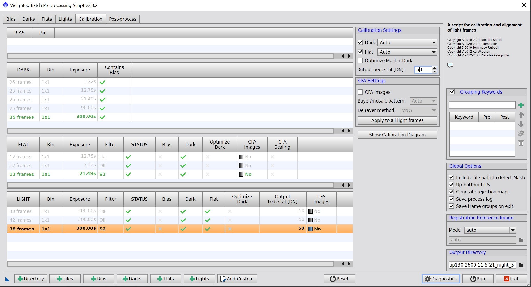
This was the basic setup for WBPP.

The Post Process view shows the summary of frames used.
3. Image Integration
Run for each filter: Ha, O3, & S2
We have a good sampling of subs so Winzorized sigma clipping with sigma low = 3.5, and Sigma high = 2.4
Psf signal used for weights
Check low and high large scale structure 2x2
This was used for all filters
4. Dynamic Background Extraction
The Ha and S2 images were almost completely filled with nebula and no gradients were seen, so I. elected not to run DBE on these masters.
A gradient is only seen on the O3 Master so DBE was run on this image.

The DBE sampling pattern used on the O3 master image
The O3 Master image before DBE. (click to enlarge)
The O3 Master Image after DBE has been applied - note how much flatter it is. (click to enlarge)
5. Deconvolution Prep
For all images
Object mask created
A nonlinear version of the image was created using STF->HT
Use HT to clip blacks and push stars and nebula to white
Create Local protection images
Run StarMasks with layers = 6, all else default
Adjust star mask with HT to boost star size - move the middle arrow to the 25% point
Create PSF image with PSFImage Script.
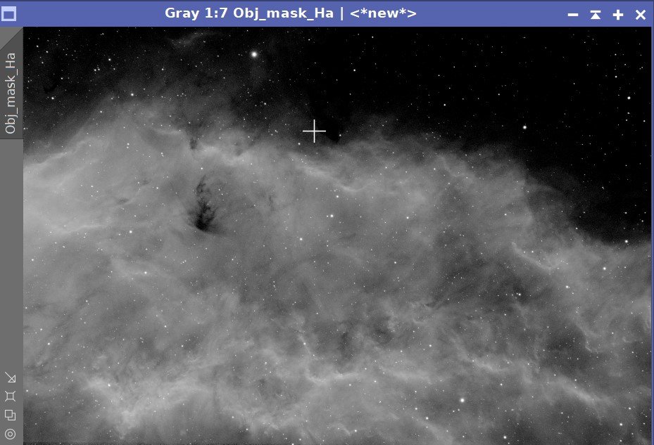
Object Mask for Ha

Object Mask for O3

Object Mask for S2

PSF image for Ha
Ha Local Support Image (click to enlarge)

PSF image for O3
O3 Local Support Image (click to enlarge)
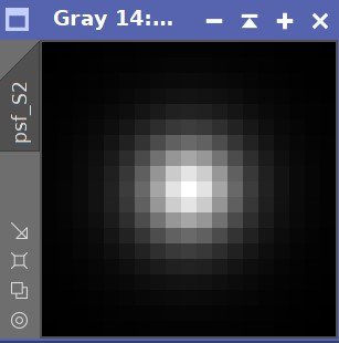
PSF Image for S2
S2 Local Support Image (click to enlarge)
6. Apply Deconvolution
For all images:
Apply Object mask to the image
Set psf to the right one for the image
add the right local support image
Create 3 preview sections on the image
Test different global dark settings until optimal found
Ha - 0.007
O3 - 0.006
S2 - 0.006
Ha image before deconvolution. (click to enlarge)
O3 image before deconvolution. (click to enlarge)
S2 image before deconvolution. (click to enlarge)
Ha image after deconvolution. Stars are smaller and detail is a bit shaper (click to enlarge)
Ha image after deconvolution. Stars are smaller (click to enlarge)
Ha image after deconvolution. Stars are smaller and detail is a bit shaper (click to enlarge)
7. Run a Light NR pass to take the “fizz” off each image.
Run MLT DeNoise (See panel image below for settings)

This is a sample from the Ha image. The image has low noise. (click to enlarge)

This is after MLT NR. much cleaner. (click to enlarge)
This sample is from the O3 image - the noise level here is much higher. (click to enlarge)
After MLT NR. Much better! (click to enlarge)
The S2 image before MLT NR. (click to enlarge)
S2 image after MLT NR. (click to enlarge)
8. Create Nonlinear Versions of the Images
For each image
Select background sky reference for each image and create a preview for them
Run MaskedStretch using the preview of each image for the background reference.
Run CT for each image and adjust the tone scale to get a good-looking image. Try to balance the backgrounds to be consistent.

Liinear images: Ha, O3 and S2 - after decon and NR.

The Nonlinear Images: Ha, O3, and S2
9. Create Color Image
Run Chanel combination tool with new Nonlinear images to create the first color image.
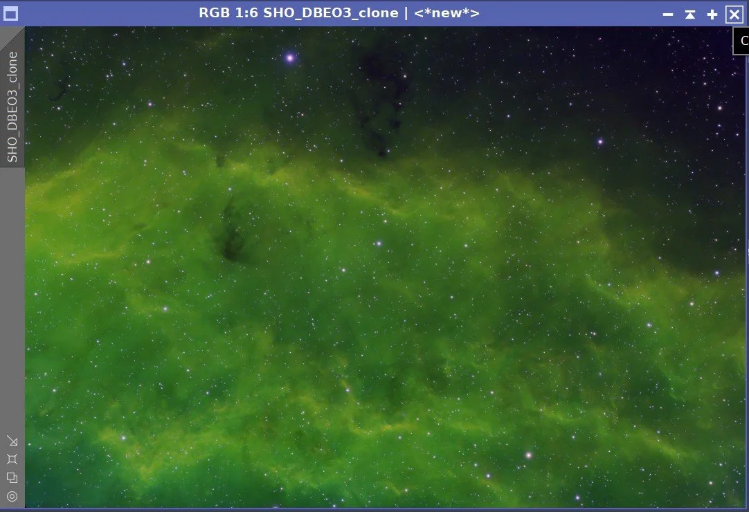
10. Initial Process of the Color Images
Use SCNR to remove the Green from the initial Image
Invert the Image, run SCNR again to remove green, and then Invert the image back. This removes residual magenta tones.
Use CT to tweak tone scale and saturation
Create a blue mask using the ColorMask script - removing 2 layers to blur. Use HT to boost
Break blue mask into two sections
Copy the blue mask.
On one copy, use the DynamicPaintBrush to eliminate stars and star rings from the mask
In the other copy, use he DynamicPaintBrush to eliminate everything BUT stars and star rings from the mask
Apply Blue Star mask to image and use CT to reduce blue color around stars and reduce sat
Apply Blue No-Star mask. Use CT to enhance blue areas of the nebula
Create a Green mask using the ColorMask script - removing 2 layers to blur. Boost with HT.
Apply Green mask to SHO image, and boost Red layer, adjust Blye layer, and boost sat.
Apply Local Histogram Equalization with a radius of 130 max contrast of 2.0, and amount of 0.16, 10-bit histogram.
Apply Local Histogram Equalization with a radius of 260, max contrast of 2.0, and amount of 0.08, 10-bit histogram
CT run to enhance lower-end contrast
FInally - rotate the image to get a better composition.
TThe Color image after the SCNR-Invert-SCNR-Invert process (click to enlarge)
Aftre the first CT to adjust tone scale and saturation (click to enlarge)
The Beginning Blue Mask (click to enlarge)
Blue Mask with Nebula removed. (click to enlarge)
Blue Mask with Stars removed. (click to enlarge)
The Green Mask - which maps niceling on the gold regions.

After Blue Star Mask applied and saturation adjusted

After Green mask fixes, LHE adjustmets and Image Rotation
12. Nonlinear Noise Reduction
Use ACDNR to do a Nonlinear Noise Reduction. Use parameters shown in the panel images below.

ACDNR Lightness Parameters

Before ACDNR Applied.

ACDNR Chrominance Parameters

After ACDNR Applied.
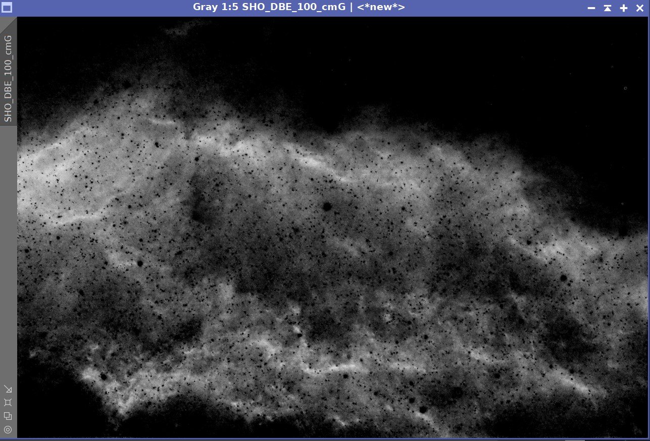
13. Enhance Dark Structures
run EnhanceDarkStructures Script with the amount set to 0.35
14. Crop Images
I saw a somewhat ragged edge at the top of the image so I ran a slight Crop.
15. Star Reduction
Run EZ-StarReduction using everything default and the Adam Block Method.
Before running EZ-StarReduction. (click to enlarge)
After Running EZ_StarReduction (click to enlarge)
16. Save images as Tiff and Move to Photoshop
In Photoshop:
Use Camera Raw Filter to adjust Global Clarity, Texture, and Color Mix
Use StarShrink filter to reduce large stars radius 35 strength 6, sharpness -1
Use StarShrink filter to reduce small stars radius 2, strength 6, sharpness -1
Using Lasso with a father of 150 pixels, select dark regions, and other regions of interesting detail and boost clarity and curves.
Use healing brush to fix some stars with desaturated halos around them.
Add watermarks
Export Clear, Watermarked, and Web-sized Jpegs.
Capture Details
Lights Frames
Taken the nights of November 5th-8th, 2021
40 x 300 seconds, bin 1x1 @ -15C, Gain 100.0, Astrodon 5nm Ha Filter
42 x 300 seconds, bin 1x1 @ -15C, Gain 100.0, Astrodon 5nm OIII Filter
38 x 300 seconds, bin 1x1 @ -15C, Gain 100.0, Astronmiks 6nm SII Filter
Total of 10.0 hours
Cal Frames
25 Darks at 300 seconds, bin 1x1, -15C, gain 100
25 Dark Flats at Flat exposure times, bin 1x1, -15C, gain 100
Flats darks
12 Ha Flats
12 OIII Flats
12 SII Flats
Capture Hardware
Scope: Astrophysics 130mm Starfire F/8.35 APO refractor
Guide Scope: Televue 76mm Doublet
Camera: ZWO AS2600mm-pro with ZWO 7x36 Filter wheel with ZWO LRGB filter set, Astrodon 5nm Ha & OIII, and Astronomiks 6nm SII Narrowband filter set
Guide Camera: ZWO ASI290Mini
Focus Motor: Pegasus Astro Focus Cube 2
Camera Rotator: Pegasus Astro Falcon
Mount: Ioptron CEM60
Polar Alignment: Polemaster camera
Software
Capture Software: PHD2 Guider, Sequence Generator Pro controller
Image Processing: Pixinsight, Photoshop - assisted by Coffee, extensive processing indecision and second-guessing, editor regret and much swearing…..
Adding the next generation ZWO ASI2600MM-Pro camera and ZWO EFW 7x36 II EFW to the platform…