
IC 1396A - The Elephant’s Trunk - 7.3 hrs in SHO (a Case of Virus Interuptus)
Date: Nov 2, 2022
Cosgrove’s Cosmos Catalog ➤#0113
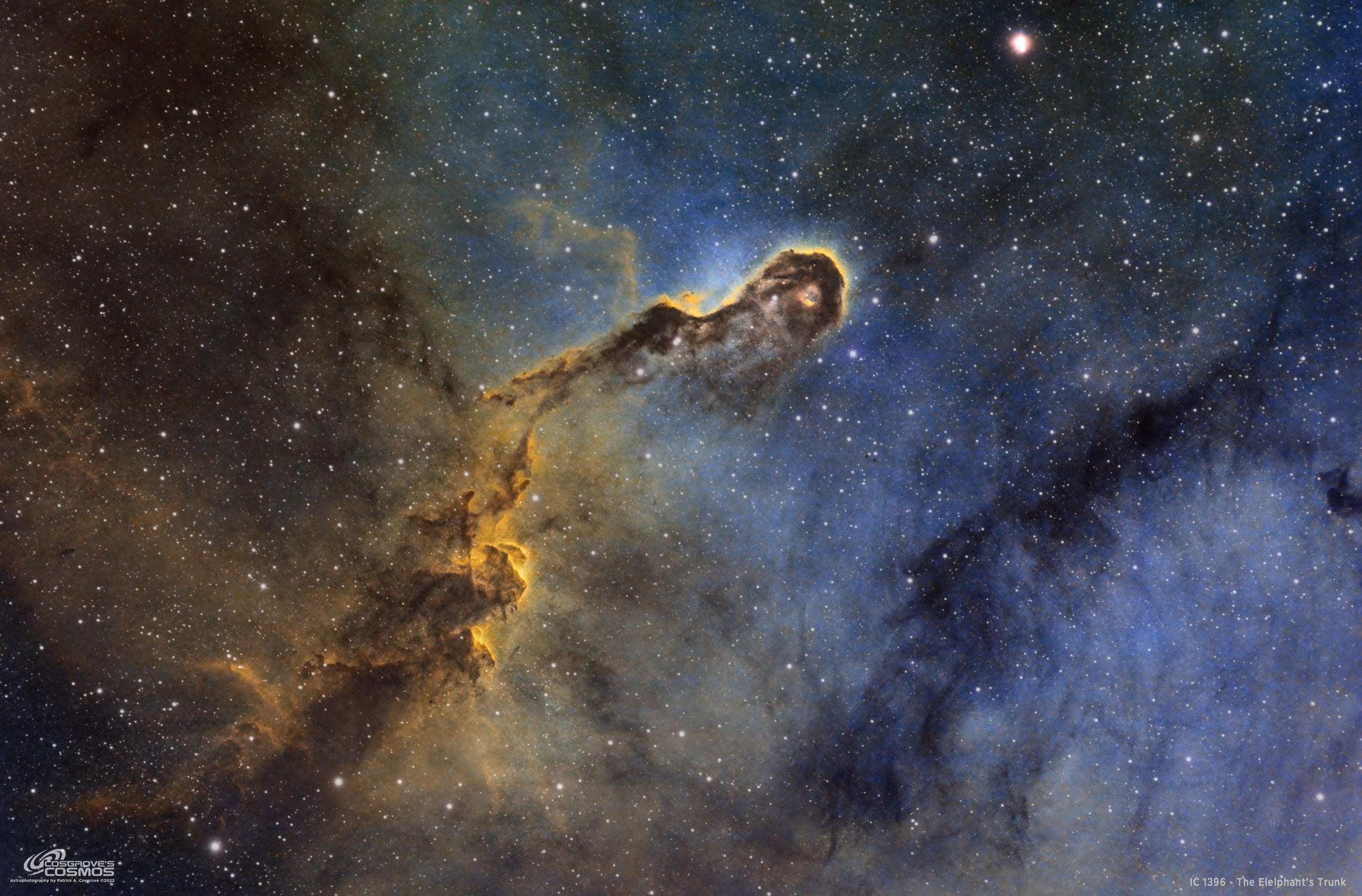
IC 1396A - The Elephant’s Trunk Nebula - imaged with my Astro-Physics 130mm f/8.35 refractor, A ZWO ASI2600mm-Pro camera, and a Ioptron CEM60 mount. (click for full resolution via Astrobin.com)

Granted “Explore” Status on Flickr!
This image was published in Amateur Astrophotography Magazine, in their Issue #106, Nov 2022, , on pages 72-73!


Table of Contents Show (Click on lines to navigate)
About the Target
This target is an old friend of mine that I have shot several times before. So I will use a description from one of my earlier postings:
IC 1396 is a large circular region of glowing gas and dust in the constellation of Cepheus and is located about 2400 light-years from Earth. Measuring approximately 100 light-years across, this region is energized by a bluish central multiple-star called HD 206267.
The ionized gas glows bright, while dark dust concentrations in the area can also be seen.
The Elephants Trunk, IC 1396A, is one feature that stands out prominently in images taken of the area. Pressure from bright stars in the core blows dust from that area leaving behind a darker region at the center of the nebula while compressing dust around the edges, which drives new star formation. As a result, up to 250 young stars - all less than 100,000 years old, have been detected in infrared images taken of the Trunk region in 2003. The Trunk itself is about 20 light-years long.
The Annotated Image

This annotated image was created using the Pixinsight ImageSolve and ImageAnnotation scripts.
The Location in the Sky

This finger chart was created in Pixinsight using the FinderChart process.
About the Project
Intro Video
This video was added to the post a few days after it was first published. I had to recover enough that I got my voice back! So here is an overview of the image processing strategy for this image:
Choosing the Target
October brings mixed feelings for an Astrophotographer living outside Rochester, NY.
On the one hand, we are entering the realm of long dark nights with lots of opportunities for data collection. On the other hand, we are also edging into a time when clouds seem to move in and stay for months! When you have clear skies during this time of year, you are compelled to use them!
It looked like we might have a few good nights, so I made plans. I noticed that IC1396 was in a good position for me - but I have shot this before. Why shoot it again?
The first version was a short-exposure LRGB image - one of my first. The second was the same image but with Ha data added. The next version was a widefield version - an early image with my Askar FRA400 Astrograph.
But - none of these were shot:
with my newer ASI2600MM-Pro camera
as a long integration SHO project
So my goal here was to get a deep exposure at the full image scale of the AP130 platform and 2600 camera and see what I could get.
Data Capture
My plan was to capture data over the course of 3-4 nights - with the goal of acquiring about 15 hours of integration time.
We had planned a trip to visit my son’s family in North Carolina, and the dates were set such that we would get home just as the new moon was coming to fruition.
We knew the time home would be crazy. We will have been away for a few weeks, and we had some photography scheduled of the exterior of our house - should we list it later in the year as part of a plan to move and develop an observatory. We wanted to get the fall foliage into the shots. Of course, this meant a lot of work had to be done in preparation for this. Raking leaves, mowing the lawn, edging sidewalks and planting areas, and so on.
So I would work hard all day and then be up all night to catch my photos. It would not be easy - but it was doable.
Virus Interruptus
Then we had one slight wrinkle in the plan.
On our 12-hour drive home from NC, my wife ended up having a sore throat. So we were in the car together for 12 hours, you know I was going to get what she had. A couple of days later, I had a tickle in my throat as I was doing yard work and staying up all night. You just got to fight through it. Right?
Wrong!
After two days of this, I descended into the worst chest cold I had ever had. It was so bad that I felt must be COVID. (It was not.) Or it must be RSV (it was not). It was just a bad secondary infection. I could not sleep, I could not eat, and I had no energy. Suddenly the lure of the night skies was greatly diminished - hell - it was GONE!
We had two more clear nights - not that I would know it - I was sick as a dog.
Of course, my wife ended up with a slight cold for 3 days and got over it. I started a cycle that will likely last for weeks. I wish I had her immune system!
After a few days and some heavy meds, I began to recover slowly. I am still under the weather, but I managed to find enough energy to process this image and start this post!
I failed in my data collection goals - but at least this time, you don’t have to hear me complain about our weather.
But I learned an important lesson the hard way. These great targets will be there in the future. Old crotchety astrophotographers may not be if they don’t prioritize their health!
So this image resulted in subs captured over two nights - on October 21 and 22. The first night was quite breezy, and I was concerned about my tracking, but the second night was steady. A total of 7.3 hours was collected. Let’s see what we can do with the data we have!
Data Analysis
Blink analysis showed pretty clean data for each night for all filters used. The sky transparency was not great for either night but was acceptable. There were some slight gradients and a few satellite trails. Close inspection showed some subs with slightly elongated stars from the first night. Not perfect, but not horrible either. With a deep exposure, I would have considered culling some of those frames - but I was not going to be that picky given the failure to achieve a deeper integration.
Previous Efforts
Let’s take a look at those earlier efforts to image the Elephants Trunk.
The first time was on July 22, 2020, using the AP130 scope and a ZWO1600MM-Pro camera. This was an LRGB integration of 1.66 hours. This imaging Project can be seen HERE.
The second time was on July 26, 2020, just 5 days later - using the same setup, but this time I added an hour of Ha data (the first narrowband data I had ever collected at the time) for total integration of 2.66 hours. This imaging Project can be seen HERE.
The 3rd effort was made on October 26, 2021 - almost one year ago. This was an early imaging project for my smaller Askar FRA400 rig. This one was noteworthy for several reasons:
it is one that I took from a remote location (my Son’ townhouse in NC)
It was wide field - showing the entire gas cloud region
and the fact that Astronomy Magazine published this image in their September 2022 issue! That imaging project can be seen HERE.
Here are all three, side-by-side, for comparison:
2020 (click to enlarge)
2020 (click to enlarge)
2021 (click to enlarge)
Image Processing
I decided to drizzle-process this image. Why? Because I had never done this with a larger-scale image and wanted to see how it would go.
I used the automated features now built into WBPP to accomplish this, but there is. a price to be paid when doing this. First, the images are much larger and take up more storage. Second, all processes applied run slower as more pixels must be processed. But there are other things as well.
Normally I get very good results from Deconvolution at this image scale. But I have never tried applying Deconvolution when drizzled. While I tried many different techniques in my toolbox, I could not get a result that I liked. In the end, I skipped deconvolution - which is rare for me.
My go-to method for noise management - RC’s Noise XTerminator - also seems not to be as effective with drizzle images. I found I needed to be more aggressive than usual. Your mileage may vary.
My basic flow here was of a starless process:

A high-level diagram of my processing workflow
I created a synthetic luminance image by using ImageIntegration with no rejection with the Ha, O3, and S2 images.
I did minimal processing in the Linear domain and then moved all images to the nonlinear domain. Since I was planning on star removal, I just used the standard STF->HT method of going nonlinear.
At that point, I split the processing between the L and the Color image. I enhanced the detail where possible in the L image and focused on a good starting color image for the SHO.
After this, I went starless - in this case, using RC StarXTerminator for both L and SHO images. I used the L image as the basis for a stars-only image - as I don’t like the weird colors you can get in narrowband stars.
The Starless images were processed, and the L image was inserted into the SHO image using LRGBCombination. Once processing was finalized, the stars were screened back into the image. I found that no star reduction needed to be done.
I was pretty happy with the final results. I left a lot more green in the SHO image than I normally do - and the effect works well for me here I think. I also like the composition. Now, if I could have only gotten another 7 hours of data!!!
A detailed Processing Walk-Through is provided for this image at the end of the posting…
More Information
Wikipedia: The Elephants Trunk Nebula
Spitzer Space Telescope: IC 1396 in Infrared
Capture Details
Lights Frames
Data were collected over two nights: Oct 21 & Oct 22, 2022
34 x 300 seconds, bin 1x1 @ -15C, Gain 100, Astrodon 5nm Ha
32 x 300 seconds, bin 1x1 @ -15C, Gain 100, Astrodon 5nm O3
22 x 300 seconds, bin 1x1 @ -15C, Gain 100, Astronomick 6mm S2
Total of 7.33 hours
Cal Frames
25 Darks at 300 seconds, bin 1x1, -15C, gain 100
15 Flats at bin 1x1, -15C, gain 100 - for Ha, O3, S2 filters
25 Dark Flats at Flat exposure times, bin 1x1, -15C, gain 100
Software
Capture Software: PHD2 Guider, Sequence Generator Pro controller
Image Processing: Pixinsight, Photoshop - assisted by Coffee, extensive processing indecision and second-guessing, editor regret, and much swearing…..
Capture Hardware:
Scope: Astro-Physics 130mm F/8.35 Starfire APO built in 2003
Guide Scope: Televue TV76 F/6.3 480mm APO Dublet
Main Fous: Pegasus Astro Focus Cube 2
Guide Fous: Pegasus Astro Focus Cube 2
Mount: IOptron CEM60 - new
Tripod: IOptron Tri-Pier with column extension - new
Main Camera: ZWO ASI2600MM-Pro - new
Filter Wheel: ZWO EFW 7x36 - new
Filters: ZWO 36mm unmounted Gen II LRGB filters
Astronomiks 36mm 6nm Ha, OIII, & SII filters - new
Rotator: Pegasus Astro Falcon Camera Rotator
Guide Camera: ZWO ASI290MM-Mini
Power Dist: Pegasus Astro Pocket Powerbox
USB Dist: Startech 7 slot USB 3.0 Hub
Software:
Capture Software: PHD2 Guider, Sequence Generator Pro controller
Image Processing: Pixinsight, Photoshop - assisted by Coffee, extensive processing indecision and second-guessing, editor regret, and much swearing…..
Click below to see the Telescope Platform version used for this image:
Image Processing Walk-Through
(All Processing is done in Pixinsight - with some final touches done in Photoshop)
1. Blink Screening Process
Ha
pretty nice and clean data
A few trails
No frames eliminated
O3
similar to above
no frames removed!
S2
Same as above
Flats
collected each night - Data looks good
Dark flats
collected only the first night - data looks good
2. WBPP 2.5.0
Reset everything
Load all lights
Load all flats
Load all darks
Select - maximum quality
Registration reference - auto - the default
Select the output directory to wbpp folder
Enable CC for all light frames
Pedestal value - auto for all NB filters
Darks -set exposure tolerance to 0
Lights - set exposure tolerance to 0
select integration mode
Map flats and darks across nights
Setup for drizzle process

WBPP Calibration view.


The new pipeline screen for WBPP version 2.5
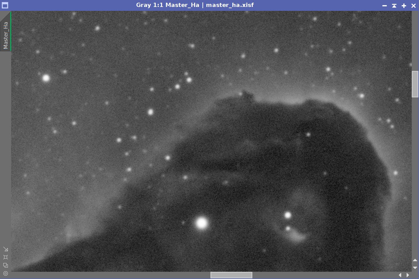
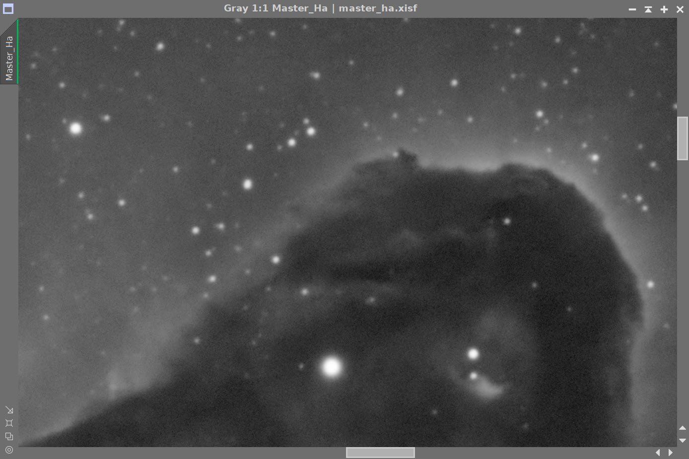
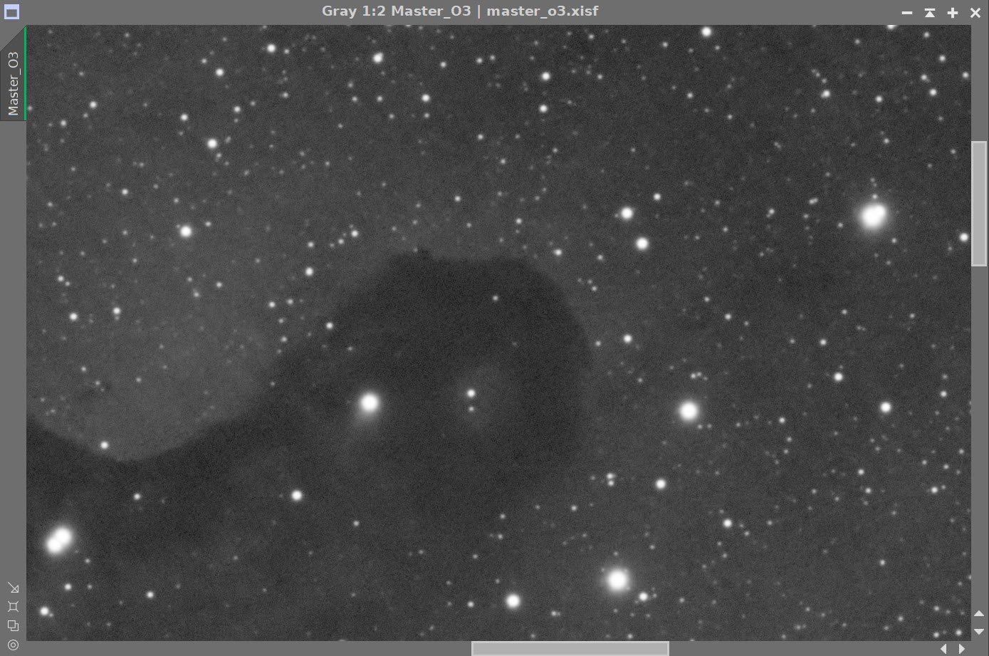
3. Load Master Images
Load all master images and rename them.
DynamicCrop was applied to all three to get rid of ragged edges
Did a 180-degree fast rotation so that the images were in the desired rotation for processing.
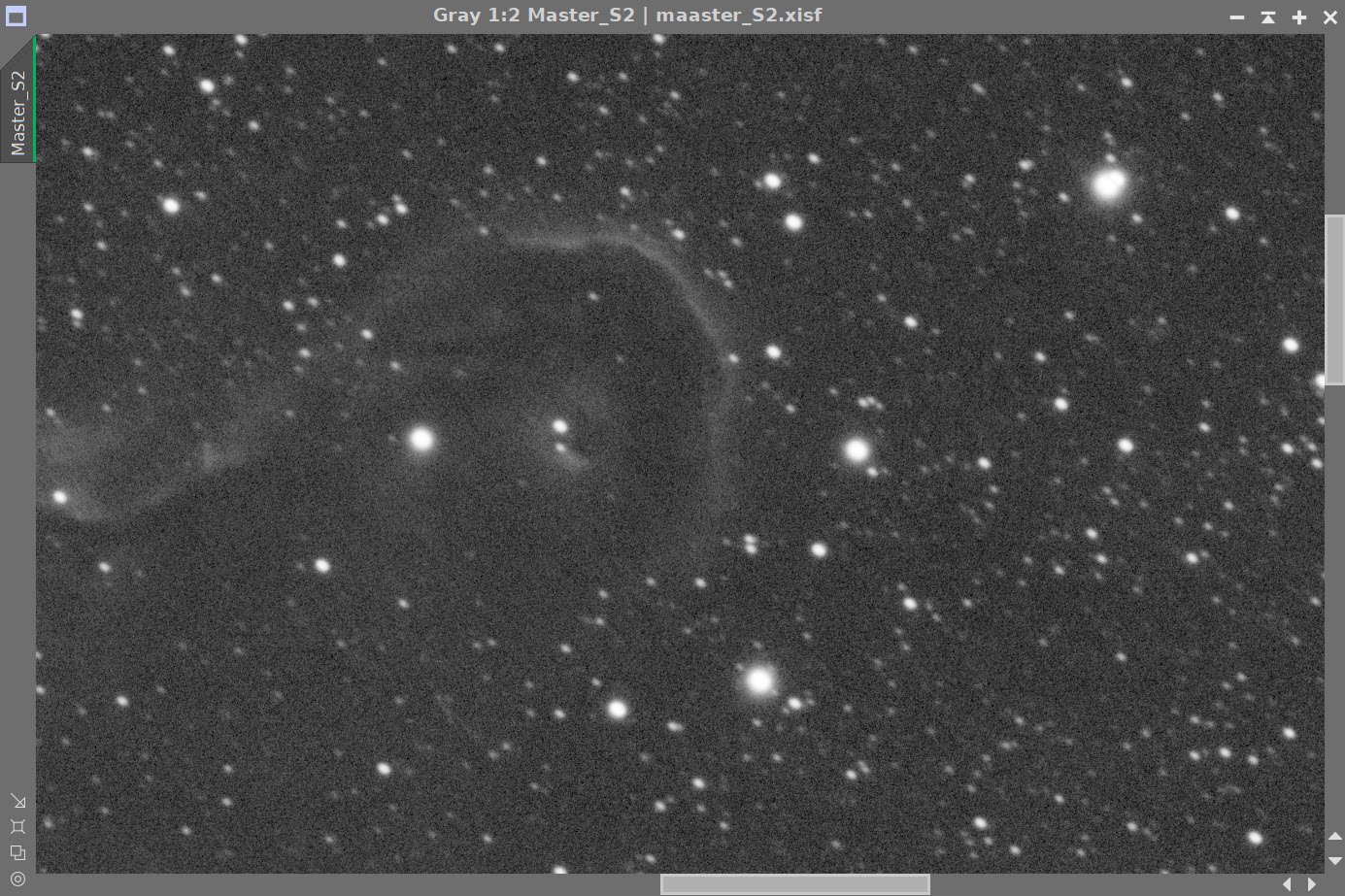
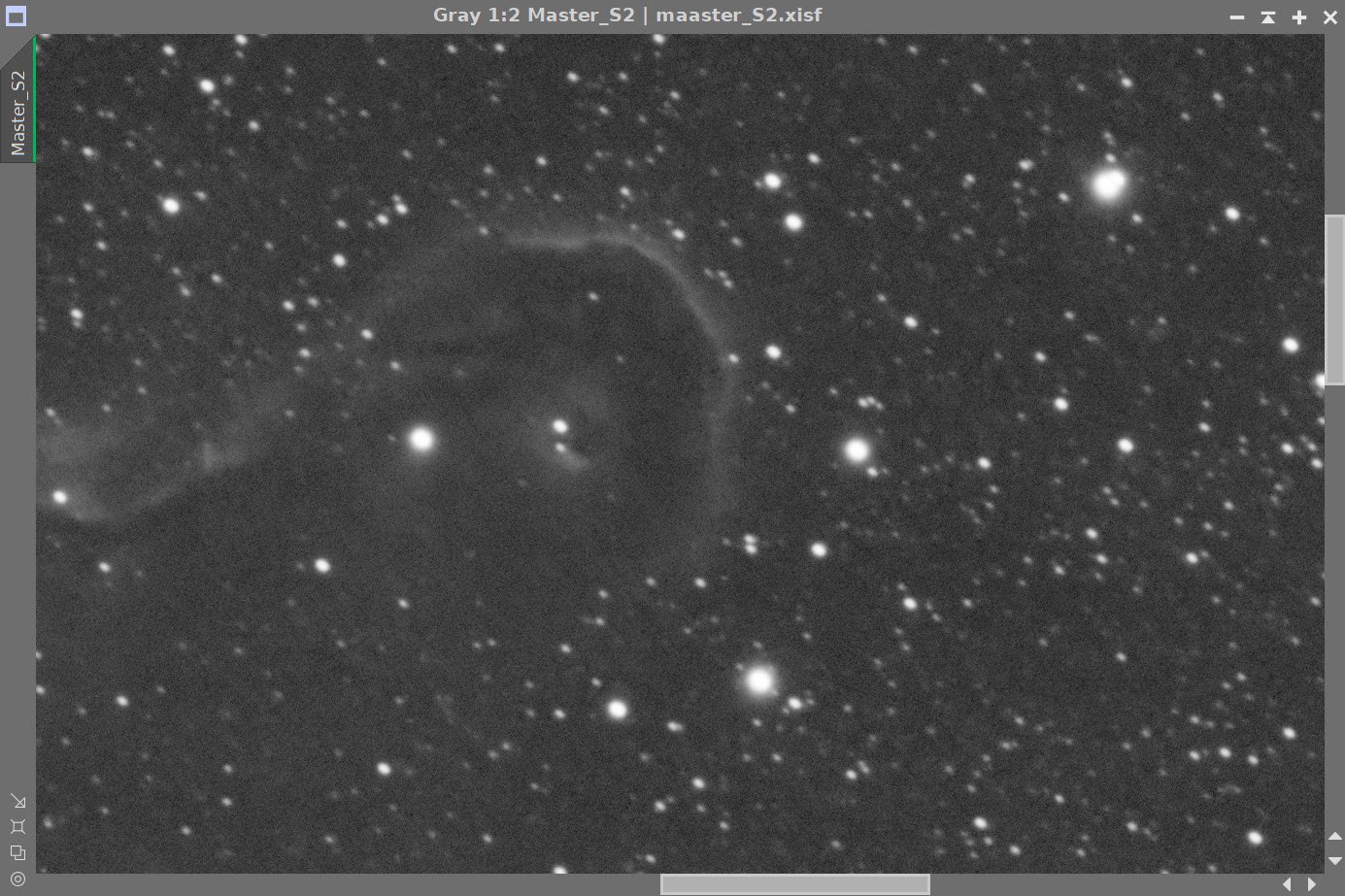
Rejection High - Ha (click to enlarge)
Rejection High - O3 (click to enlarge)
Rejection High - S2 (click to enlarge)

The initial Master Images: Ha, O3, and S2.
4. Dynamic Background Extraction
After looking at all of the nebulosity in the image and how even the fields seemed to be in general, I opted NOT to run DBE on this image. I usually do run it, so this is an exception.
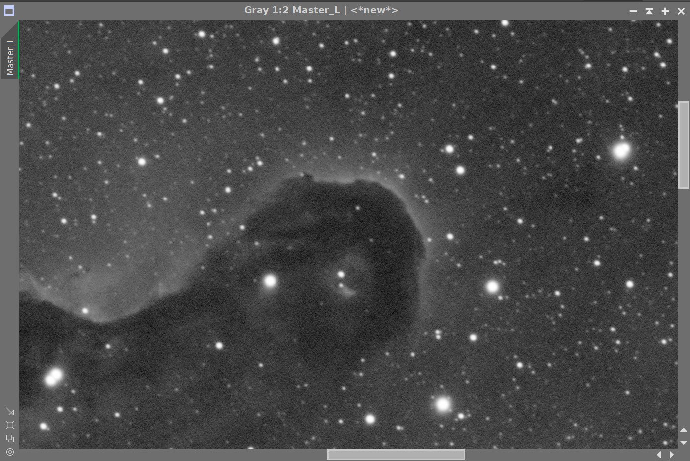
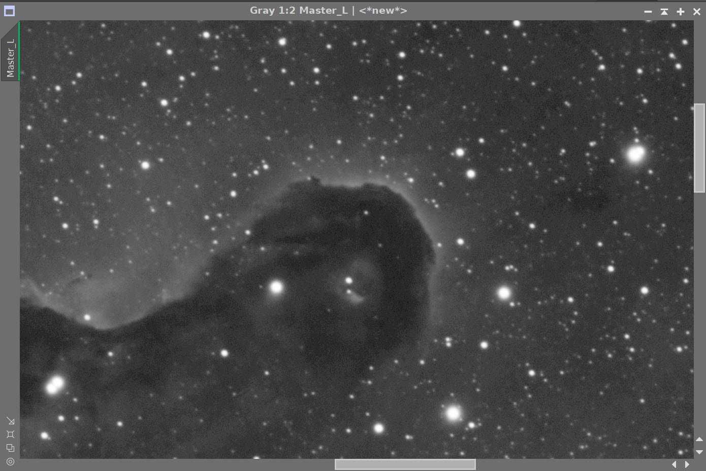
5. Create the Synthetic Luminance Image
Write the Ha, O3, and S2 Master images to files.
Run the ImageIntegration Process
Load the three master images
disable rejection
run ImageIntegration and create the Lum image
Note the weights below. Ha being the main contributor, followed by O3 and then S2 - it all makes intuitive sense.

ImageIntegration set up for creating the synthetic Lum image.

The weights used by ImageIntegration the in the creation of the new Lum image.

The Ha, O3, & S2 Master image and finally the new Lum image in the bottom right corner. This seems to be a good visual representation of all of the master images.
6. Deconvolution?
Normally at this stage, I would focus on doing sharpness restoration of the Lum image with deconvolution.
However, this is the first time I drizzle processed an image of this scale. This seemed to make a difference. No matter what I tried, I could not get a result I was satisfied with.
So for this image - no deconvolution was done.
7. Apply a Light Noise Reduction to the Master Images
Apply Noise XTerminator with a value of 0.5

Master Linear Images (Ha, O3, S2, & L) - Before and After Noise XTerminator 0.5 Linear
8. Delinearize all of the Master Images
Since my intention for this effort is to do starless processing, I will move all master images to the nonlinear domain using the standard STF->HT method. Normally this would cause star bloat, but since we will be removing stars for processing - I am less concerned with that now.

The nonlinear images.
9. Process the L Image
Using StarXTerminator create a starless and stars-only version of the image. Use the Unscreen method,

StarXTerminator Panel Set up.
L - Starless (click to enlarge)
L - Stars-Only (click to enlarge)
Using GAME, create two mask regions to cover the head and the tail of the nebula.

Apply CT to the Starless image and tweak the tone scale.

Apply “head” mask and Apply LHE with Radius=112, contrast limit = 2.0, Amount=0.5 and 8-bit histogram
The Mask used. (click to enlarge)
After the LHE application (click to enlarge)
Apply “Base” mask and Apply LHE with Radius=112, contrast limit = 2.0, Amount=0.8 and 8-bit histogram
The Mask used for this portion. (click to enlarge)
After the Targeted LHE application. (click to enlarge)
With the mask in place, Apply CT

CT is used to further enhance the snout of the trunk.
Remove mask - Apply a final CT

After the final CT tweak.
Run Noise XTerminator with 0.6
Run MLT for light sharpening.

The MLT setup used for some slight sharpening.


Before and After Noise XTerminator (0.5) and With MLT Sharpening
10. Process the Color SHO image
Examine all three nonlinear color images
Use CT to Adjust the O3 and the S2 images to have a more balanced visual appeal compared to the Ha image. This is done by eye and experience.

Original Nonlin Images

After hand tweaking with CT.
Create the first SHO color image using the ChannelCombination Tool.
Do initial color processing of the image
Apply XCNR with 75% Green Reduction
Invert the Image
Apply XCNR with 75% Green Reduction
Invert
This sequence reduces the extremes in the green and magenta portions of the image.
The initial SHO image. Lots of green because of the strong Ha signal (click to enlarge)
When you invert the image, the magenta problem turns into a green problem, which XCNR can handle. (click to enlarge)

Now XCNR is used to reduce the excess green. Here we take out about 75%. This leaves the Magenta Problem (click to enlarge)
Now we hit it with XCNR with 75% green removal. (click to enlarge)

We do a final Invert and we have the base image for our SHO color work.
Create SHO-Starless Image using StarXTerminator
Apply CT to shape the tone scale and color

Our first SHO Starless Image. (Click to enlarge)

A quick CT adjust the color and tone scale (click to enlarge)
Create Color Masks
Run ColorMask Script for Blue. This will be used to adjust the blue color tones
Do a CT Adjust to boost
Run Convolution to soften
The Initial Blue Mask (Click to enlarge)
After an adjust with CT (click to enlarge)
After several passes with Convolution (click to enlarge)
Run ColorMask Script - Green - This will be used to adjust the golden areas.
Adjust with CT
Soften with Convolution
The initial Green Mask (click to enlarge)
After a boost with CT (click to enlarge)
After softening with Convolution (click to enlarge)
Now Apply the Green Mask
Adjust color curves and sats with CT
Apply Blue Mask mask
Adjust color curves and sats with CT
After Adjust CT with the Green Mask (click to enlarge)
After Adjust CT with the Green Mask (click to enlarge)
Now Insert the L image with LRGBCombination

After Inserting L image into the SHO image.
16. Recombine Stars and Starless Images
Using PixelMath script, we will screen the L stars back into the image using the following expression:
~ ((~sho_starless_L_insert)*(~Nonlin_L_stars))

16. Star Reduction?
Typically it is at this point where I do star reduction. And I did here as well - but - to my own surprise - I did not end up using it. Why is that?
Perhaps it is because the stars were based on a synthetic L image that was heavily weighted by the Ha image. Ha stars tend to be smallish to begin with - so that might be one reason.
Another reason may be the screening method of adding stars back in. I have not used this before. One of its advantages is that it is supposed to do a better job blending the star with the surround than just adding the stars and starless images. Perhaps It changes how your eye sees things. But at the end of the day - I felt no need to reduce the star image seen here.
19. Export to Photoshop
Save the image as Tiff 16-bit unsigned and move to Photoshop
Use the camera Filter to tweak the following in a global sense:
Clarity
Curves
ColorMix
Deal with some strange pixel artifacts on the “snout. ” These od pixels seem to have come from the Noise XTerminator function. I have not run into this before. I used the blur brush to smooth them back in.
A sprinkle of pixel artifacts in the snout. (click to enlarge)
Smoothed over with the blur tool. (click to enlarge)
The left bottom Corner had a lot of blue showing at the end, So selected this area with a father of 150 pixels and cleaned it up a bit. Just a saturation reduction and slight darkening of the area.
The blue-purple corner issue. (click to enlarge)
The correction. (click to enlarge)
I tweaked some local areas with the Clarity tool
I reduced the size of the big star at the top of the frame.
And a final application of Noise XTerminator did the trick!
Finally, I added my watermarks and exported Clear, Watermarked, and Web-sized jpegs.
The FInal Image!
Adding the next generation ZWO ASI2600MM-Pro camera and ZWO EFW 7x36 II EFW to the platform…