
NGC 281 - The Pacman Nebula - 8 hours in SHO (Fighting a Strange Artifact!)
Date: Dec 3, 2022
Cosgrove’s Cosmos Catalog ➤#0116

My second attempt on NGC 281 - The Pacman Nebula. (click for high res version via Astrobin.com)
Table of Contents Show (Click on lines to navigate)
About the Target
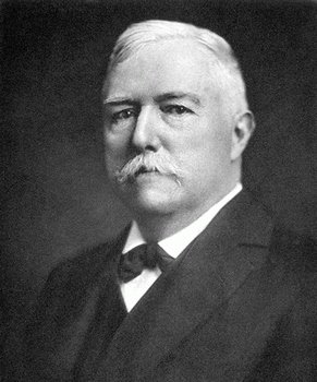
Edward Emerson Barnard (1857 -1923)
NGC 281, also known as IC 11, SH2-184, and more commonly known as the “Pacman Nebula,” is an emission nebula located 9,100 light-years away in the constellation of Cassiopeia.
This nebula measures 20 x 30 arc minutes in size and is associated with the Open Cluster IC 1590.
This object was first discovered by Edward Emerson Barnard in August 1883, who described it as "a large faint nebula, very diffuse."
The Annotated Image

This finder chart was created with the ImageSolver and FinderChart tools in Pixinsight.
The Location in the Sky

This annotated image was created using the Pixinsight ImageSolve and ImageAnnotation scripts.
About the Project
Intro Video
A few minutes of introduction for this project by yours truly! While this project posting is quite detailed, the video allows me to discuss some aspects of the project in a more personal way.
Choosing the Target
This is the fourth target I have processed from my capture session in late October.
I was away from home for a few weeks with plans on returning home just in time to start the next capture cycle. With longer nights, I had planned on capturing two waves of targets for each scope - and I made my plan accordingly.
As I looked for what targets would be well positioned for me (and my tree line), I saw that the NGC 281 would be within reach from about 9 pm until about 4 am.
I had shot this target before, but I thought it would be a good one to revisit, this time using my Astro-Physics 130mm platform using the ZWO ASI2600MM-Pro camera.
I planned to shoot this target in the earlier evening and shift to a different target around 1:30 am.
If you have seen the post for my previous three projects, then you know that I came home from my trip with a very bad cold. This cold worsened during the first two nights of capture until things got really bad for me. It evolved into the worst respiratory and sinus infections that I think I ever had in my life.
It was so bad that everything just stopped - for weeks.
This cost me two beautiful clear nights when I could have captured more photons - but that was just not in the cards!
As I processed the projects from this capture session, I delayed processing this one, as I was short data with the S2 filter.
A month went by, and I finally had a clear evening open up on November 23rd, and I used it to supplement data for this project.
Data Capture
Most of the subs were captured over the nights of Oct 21 and 22, with a final night of capture on Nov 23rd.
In general, these nights were clear and very cool. The first night was a bit breezy, and I was concerned about my guiding given that my scopes are in the driveway and exposed - but the guiding stats looked good, and the subs showed good star images. I did not think either night was particularly transparent - but my subs seem to be looking reasonable, and I was satisfied.
The final night was very clear and very cold. When I shut things down, I had a heavy build-up of frost on all of my equipment!
Data Analysis
Blink analysis showed that the data looked pretty solid for all filters. No subs needed to be removed. I ended up with just a bit over 8 hours of narrowband data.
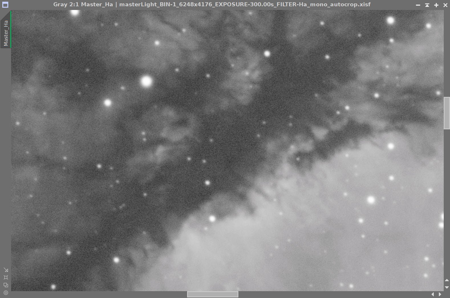
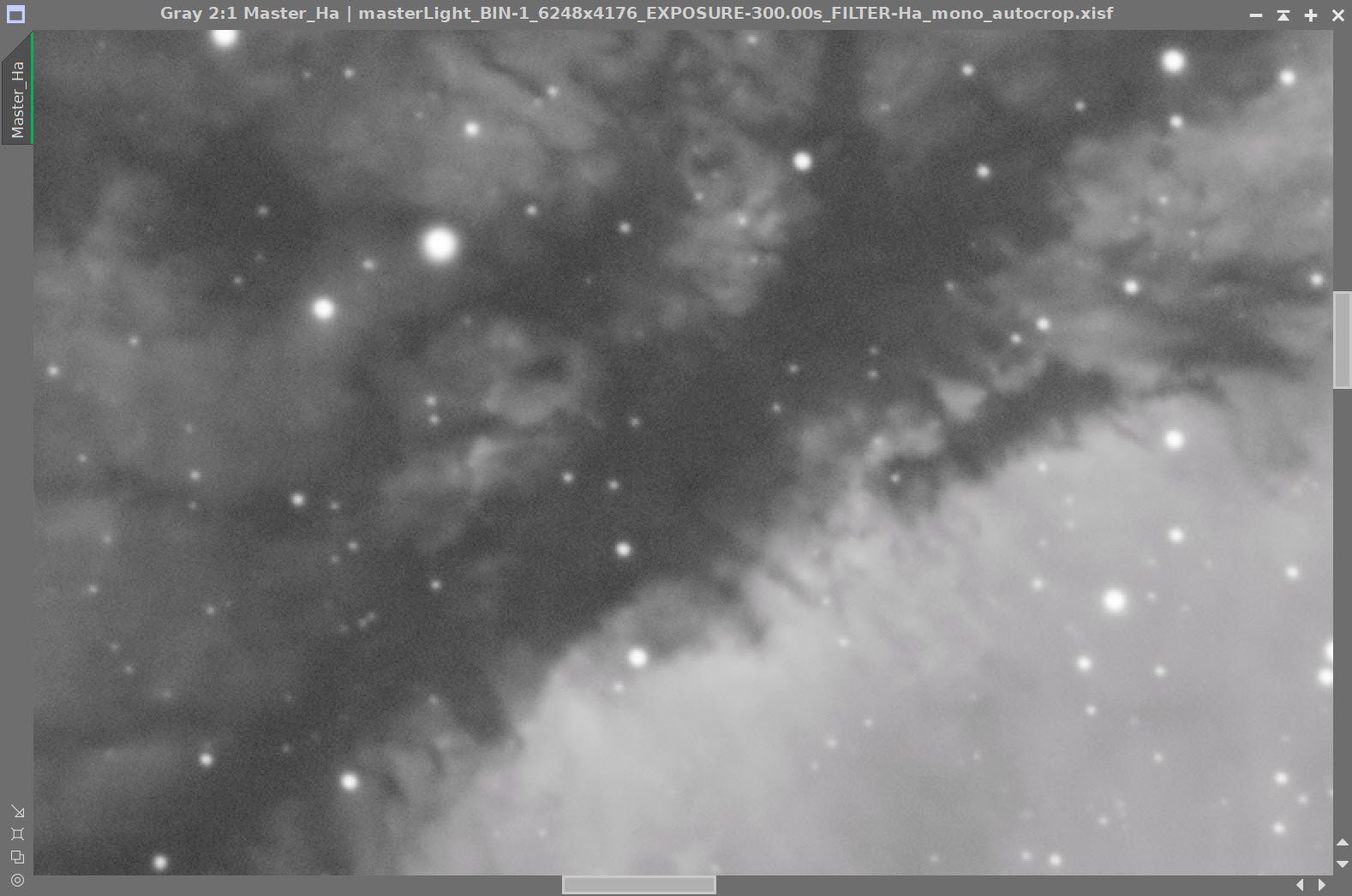
When I first did my blink analysis, I did not notice a nested ring-like artifact in the lower left-hand corner of the screen. Subsequently, I went back and saw that this artifact is visible here as well an was a constant feature across all o the subs. I will talk more about this later.
Previous Efforts
As I indicated, I have shot this target once more in the past - back in November of 2020. This was a 6.8-hour narrowband exposure in SHO, using the same telescope platform - but at that time, it was sporting a ZWO ASI1600MM-Pro camera. You can see that project posting HERE. You can see that image below - along with the current one, for comparison. This was a fairly early narrowband SHO image for me, and I must say - I don’t think I did too badly with it! It was a fairly long integration time, and the processing brought out a lot of details in the nebula.
Having said that, I find that I like the new version much better. The colors are richer, there is more detail, and the whole target seems more three-dimensional to my eyes. The only thing I don’t like better is how dark I ended up making the background sky - this was caused by the need to deal with the low-signal artifact. While this dark background is not my normal processing preference - it does seem to make the image pop a bit!
NGC 281 - taken in Nov 2020 (click to enlarge)
NGC 281 - our current image (click to enlarge)
Image Processing
This project, just like the last few, is an SHO narrowband capture with 5-minute subs. It follows my standard workflow for these kinds of images - as can be seen in the chart below.

The processing flow for this project.
However, there were a couple of significant differences here that I would like to call out.
Strange Image Artifacts
I found a strange set of artifacts that I have never seen on an image before. Note the red rings and the strange red noise pattern in the image below:

The strange ring artifacts and mottling I encountered on this image!
While it looks like a red artifact, it is not. With some investigation, this is what I found:
The pattern is seen on every master image. (So it is not a filter-specific artifact)
No such pattern was found in the flat masters or the flat subs. (So it was not introduced with the flats)
No pattern was found in any of the darks (So this was not introduced via calibration)
The pattern is seen in both master images and raw subs. (So it is in the Light data and is not a pre-processing artifact)
The pattern is seen in all of the subs (so it was not introduced by some local light source causing reflections in the system).
This was very strange. In my three years of practicing astrophotography, I have not run into anything like it.
Right now, my best theory is that this was interreflections in the system introduced by the bight star Alpha Cas (Schedar) - which is near this target - along a vector from the center of the image to the rings seen in the corner. While the bright star is not in the sensor FOV, it could be just inside the scope FOV and causing halos or reflections. I am not sure.

Here is a screen shot from Stellarium showing Alpha Cas and it proximity to NGC 281.
Have you seen an artifact like this before?? Do you have any ideas on what caused this? If you do, please leave a comment or send me a note - it would be greatly appreciated!
Have I ever seen a pattern like this before? As I thought about it - it came to me!
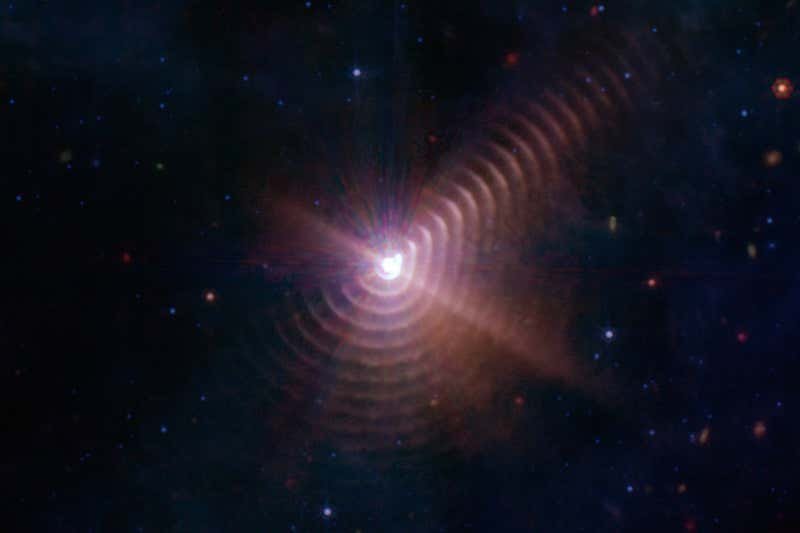
Concentric rings of dust spreading away from a star system called WR 140
NASA/ESA/CSA/STScI/JPL-Caltech
The James Webb Space Telescope recently shared this image of concentric dust rings found around a Wolf-Rayet Star known as WR 140!
Clearly - my little telescope was matching the performance of the JWST! This was not an artifact - it si a new discovery! Yeah - right. Nice try, Pat!
This unknown artifact certainly caused me a lot of problems in processing. I tried a lot of things to mitigate the problem - but at the end of the day, I ended up having to hide in the blacks. As a result, my image has a much darker background than I would usually use. This is very frustrating since the high signal areas of the image look quite good. Some day when I have more time, I will come back to this data and see if I can find a better way to deal with this problem.
A Change in Workflow
In my normal workflow, I take the Master Ha, O3, and S2 images nonlinear, tweak them one-to-another, and then combine them to create a nonlinear SHO image. This image must then be adjusted to deal with the strong green colors you get when strong Ha images are mapped to the Green channel in the SHO mapping. This workflow has worked very well for me.
However, I saw that Bill Blandshan has created some new Pixelmath Scripts that manage the normalization of SHO images, and I wanted to try this out.
To use this script, you combine the linear master images into a linear SHO color image. You then take this image starless and apply his script. As with most of his scripts, there are a few parameters that you can adjust to change how the script operates. But with one button push, you have a normalized SHO image. This sounded very attractive.
So for this project, I adopted this change in workflow. The results were quite good - the only problem was that the color position it produced tended to highlight my artifact issue - but that is not the script's fault. I was pretty happy with this tool, and I plan on using it for my future projects. You can learn more about it in the video below:
High Color vs. Mid-Color Results
I tend to be a high-color kind of guy. By this, I mean that my natural tendency and preference is to process my images to have a higher color saturation and create images with a lot of punch.
But I sometimes am guilty of taking this too far. When I think I may have done that, I create a second image where I back off on contrast and color saturation and then offer both images up for feedback. I value this feedback, and it often helps me to finalize my image.
I felt I may have gone too far with this image, so I sought feedback.
Here are the two image options I prepared:
Here was my High-Color Version. (click to enlarge)
And here is my Mid-Color version of the image. (click to enlarge)
The high-color image had wonderfully bold blues and orange/yellow tones. With the darker-than-normal background (thanks to the ring artifacts), I thought the image had a lot of punch.
The mid-color image is more understated - and I thought the softer tones helped to highlight the dust areas a bit. But what would others think?
First, I shared this with my local brain Trust - two local astrophotographers named Dan Kuchta and Gary Opitz. One liked the mid-color image, and the other thought that something between the two would be optimal.
I then posted this on Twitter:
The old "high color vs low color" question!
— 🔭Cosgrove's Cosmos💫 (@CosgrovesCosmos) November 28, 2022
Which do you like better?#astrophotography pic.twitter.com/iAwxMZOx2X
This generated a lot of feedback. Many people liked the high-color image - but more people liked the mid-color more. At the time of this writing, I have 17 votes for the high-color version and 42 votes for the mid-color version! That’s more than 2-to-1 in favor of rolling back the color!
I’d say that was a pretty strong signal! So my final image embraced this feedback! Thanks to Dan, Gary, and the Twitter #Astrophotography community!
Please remember that there is no right or wrong here - just personal preferences. I think I will end up with many image projects where I process what I seem to like first and then offer a slightly more subdued version!
Results
The last section talked about color and contrast, but how do I feel about the final image? Well, I am super disappointed about the image artifacts that ended up in this image. I wish I understood how they came about, and I wish I had a better way of mitigating their effects. I really don’t like driving the background as dark as I had to here.
But despite that, I personally kind of like where the image came out. I captured a lot of detail within the nebula and around the dark dust lanes. Though subdued, I like the color of this image much more than what I did in my first attempt!
A detailed Processing Walk-Through is provided for this image at the end of the posting…
Capture Details
Lights Frames
Data were collected over two nights: Oct 21 & 22, and Nov 23.
38 x 300 seconds, bin 1x1 @ -15C, Gain 100, Astrodon 5nm Ha
27 x 300 seconds, bin 1x1 @ -15C, Gain 100, Astrodon 5nm O3
32 x 300 seconds, bin 1x1 @ -15C, Gain 100, Astronmiks 6nm S2
Total of 8 hours 5 minutes
Cal Frames
25 Darks at 300 seconds, bin 1x1, -15C, Gain 100
15 Flats at bin 1x1, -15C, Gain 100 - for Ha, O3, & S2 filters
25 Dark Flats at Flat exposure times, bin 1x1, -15C, Gain 100
Software
Capture Software: PHD2 Guider, Sequence Generator Pro controller
Image Processing: Pixinsight, Photoshop - assisted by Coffee, extensive processing indecision and second-guessing, editor regret, and much swearing…..
Capture Hardware:
Scope: Astro-Physics 130mm F/8.35 Starfire APO
built in 2003
Guide Scope: Televue TV76 F/6.3 480mm APO Dublet
Main Fous: Pegasus Astro Focus Cube 2
Guide Fous: Pegasus Astro Focus Cube 2
Mount: IOptron CEM60 - new
Tripod: IOptron Tri-Pier with column extension
Main Camera: ZWO ASI2600MM-Pro
Filter Wheel: ZWO EFW 7x36
Filters: ZWO 36mm Gen II LRGB filters
Astronomiks 36mm 6nm Ha, OIII, & SII filters
Rotator: Pegasus Astro Falcon Camera Rotator
Guide Camera: ZWO ASI290MM-Mini
Power Dist: Pegasus Astro Pocket Powerbox
USB Dist: Startech 7 slot USB 3.0 Hub
Software:
Capture Software: PHD2 Guider, Sequence Generator Pro controller
Image Processing: Pixinsight, Photoshop - assisted by Coffee, extensive processing indecision and second-guessing, editor regret, and much swearing…..
Click below to see the Telescope Platform version used for this image:
Image Processing Walk-Through
(All Processing is done in Pixinsight - with some final touches done in Photoshop)
1. Blink Screening Process
Ha
Solid data. No trails, no gradients
No removals
O3
Same - no removals
S2
One trail, some minor gradients
Nothing removed
Flats
Flats - night 1: looks good!
Flats - night 2:
Only one flat for Ha! This was removed - I’ll have to use flats from another night.
Some flats seemed to stick out. Two outliers were removed.
Flats - night 3:
again saw strange variants in ha and o3, and two were removed.
S2 was fine
Dark flats
Looks good
Darks
300-second darks all looked good.
I am not sure why I am suddenly seeing more variations in the flats. It was very cold, and I wonder if the panel I am using gets a little strange in the cold. In the future, I will increase my sample size for flats on cold nights.
2. WBPP 2.5.4
Reset all
Load all lights
Load all flats
Load all darks
Select peak quality
Keyword “Night”
Ref image - auto
Output folder wbpp
Set Darks exposure threshold to 0
Set Lights exposure threshold to 0
Disable astrometric solution
Map missing flats
Map missing dark flats
Set the Pedastal image to auto for all filters
Set cosmetic correction or all frames
Enable Linear Defects Correction
Enable Integration
Set Autocrop
Executed in 29.25 minutes - no errors

WBPP Calibration view.

WBPP Post-Calibration View

The new pipeline screen for WBPP version 2.5
3. Load Master Linear Images
Load the resulting Master Linear image and rename them.
Rejection High - Ha (click to enlarge)
Rejection Low - Ha (click to enlarge)
Rejection High - O3 (click to enlarge)
Rejection Low - O3 (click to enlarge)
Rejection High - S2 (click to enlarge)
Rejection Low - S2 (click to enlarge)
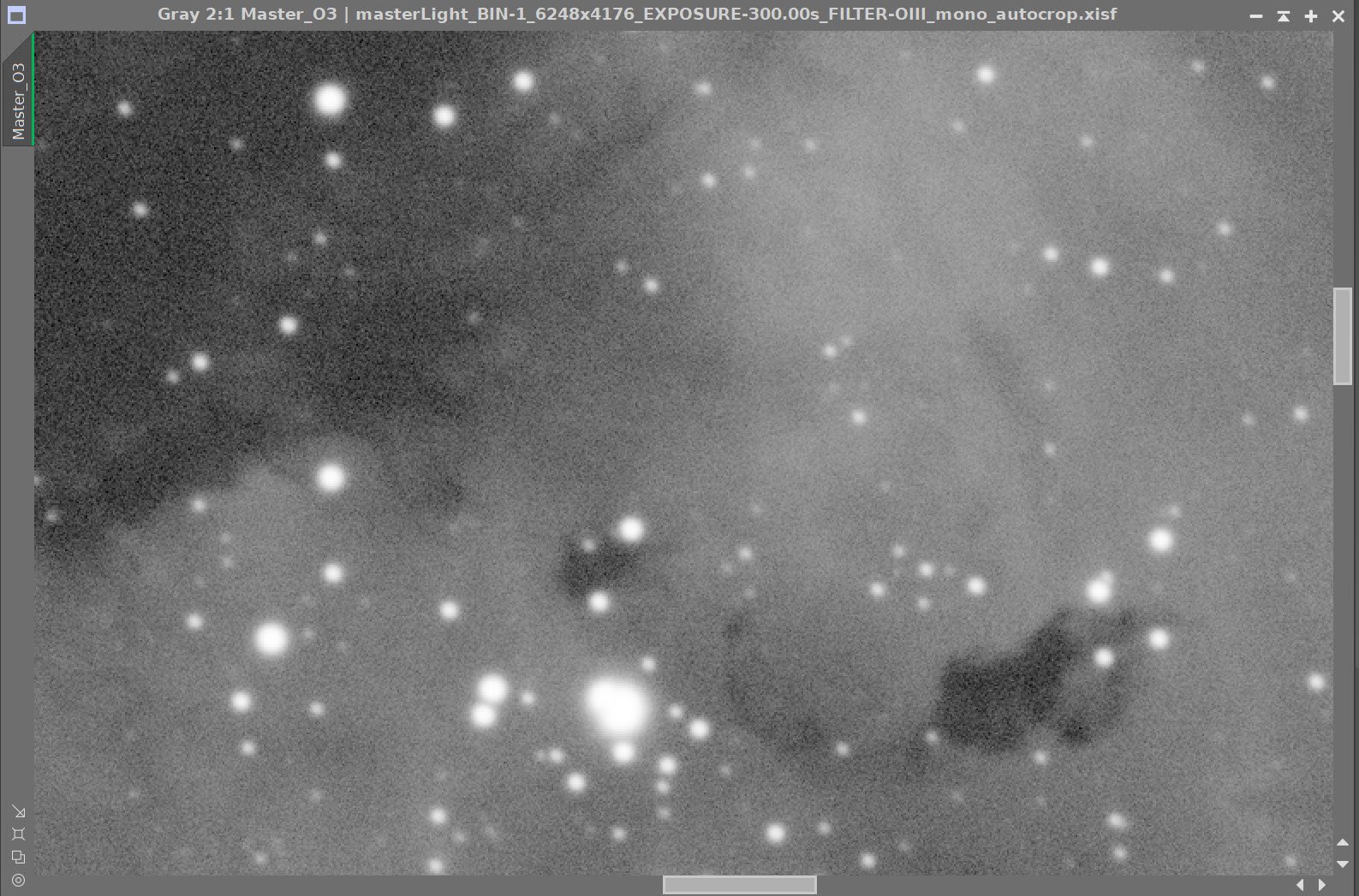
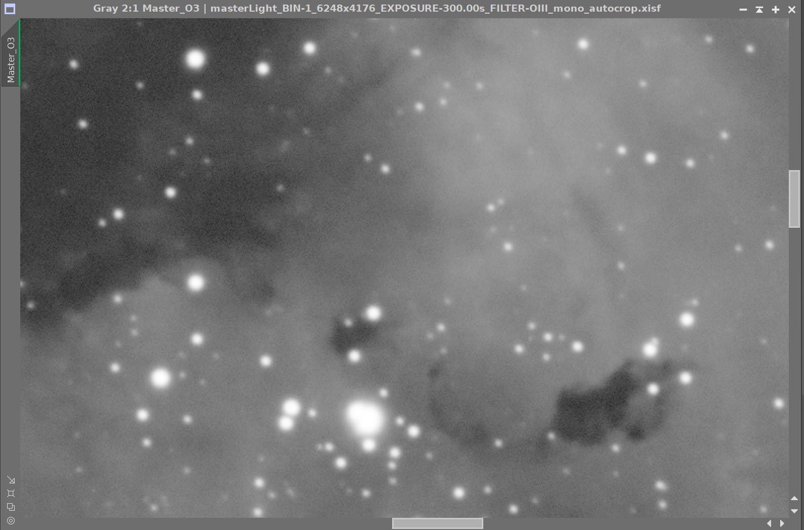
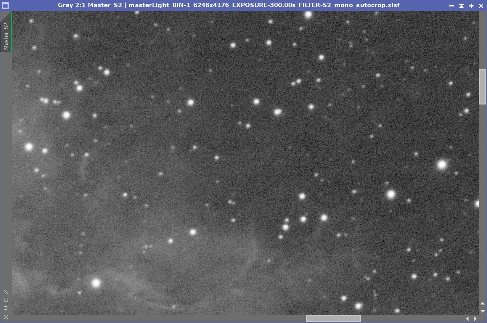
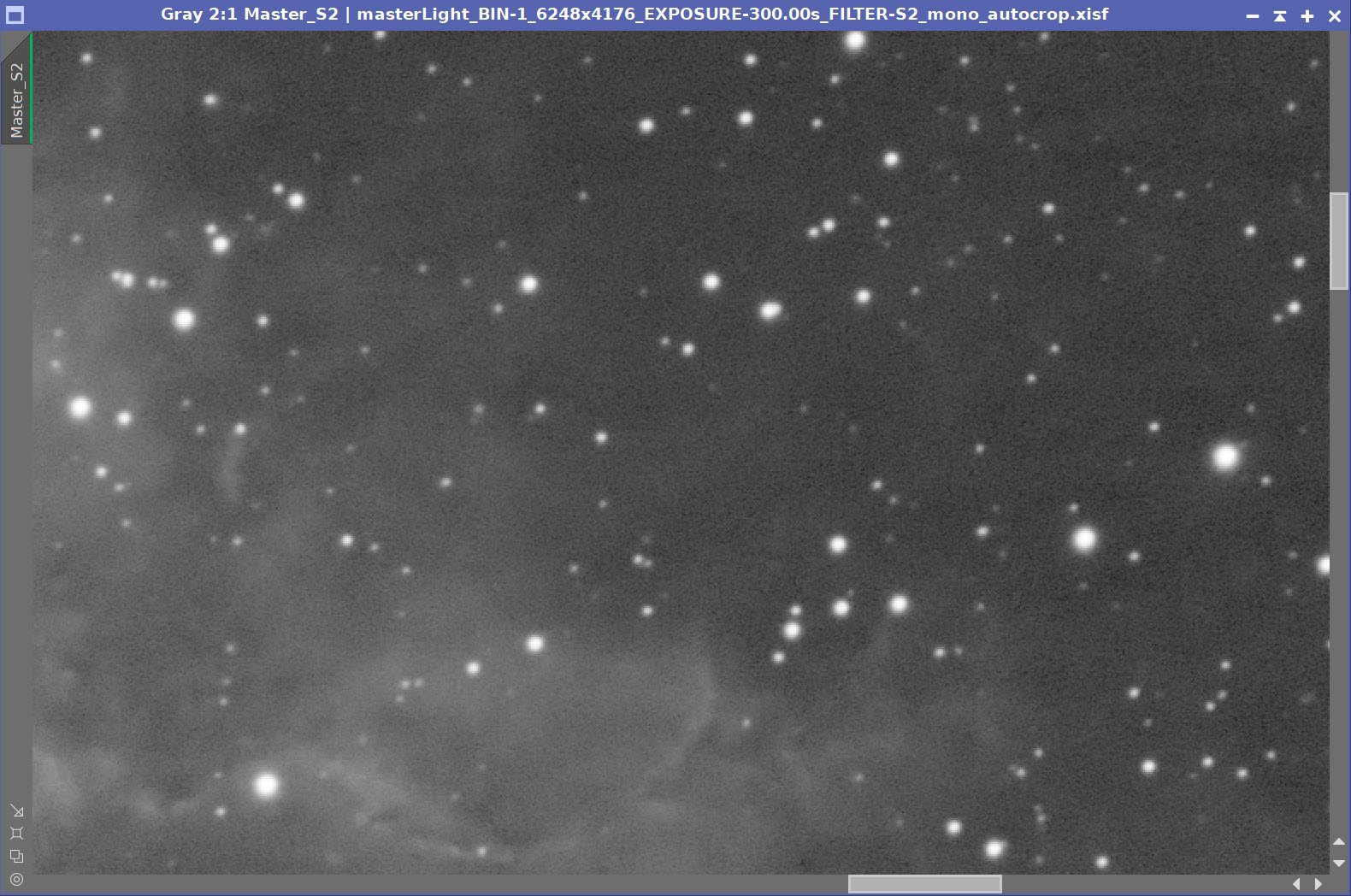
Master Ha (click to enlarge)
Master O3 (click to enlarge)
Master S2 (click to enlarge)
4. Dynamic Background Extraction
DBE applied to all images
DBE Sampling for Ha (click to enlarge)
DBE Sampling for O3 (click to enlarge)
DBE Sampling for S2 (click to enlarge)
Ha - Before DBE (click to enlarge).
O3 - Before DBE (click to enlarge).
S2 - Before DBE (click to enlarge)
Ha - After DBE applied (click to enlarge).
O3 - After DBE applied (click to enlarge)
S2 - After DBE (click to enlarge)
Ha - Background extracted (click to enlarge)
O3 - Background extracted (click to enlarge)
S2 - Background extracted (click to enlarge)
5. Apply light Noise Reduction to the Ha, O3, and S2 Linear Master Images
Ha: Apply Noise XTerminator with a value of 0.5, detail of 0.20
O3: Apply Noise XTerminator with a value of 0.6, detail of 0.20
S2: Apply Noise XTerminator with a value of 0.6, detail of 0.20
Master Linear Images - Before and After Noise XTerminator
7. Create the Synthetic Lum image and Finish The Linear Processing On It
We have three master images, which means we can use ImageIntegration to create the Synthetic Luminance Image.
I saved the three master images to disk.
I set up ImageIntegration to use those files, averaging for integration, and disabled rejection.
Run and rename the new Luminance image.

ImageIntegration Panel as used to create the Synthetic Lum image.

The weights computed by ImageIntegration to combine the images
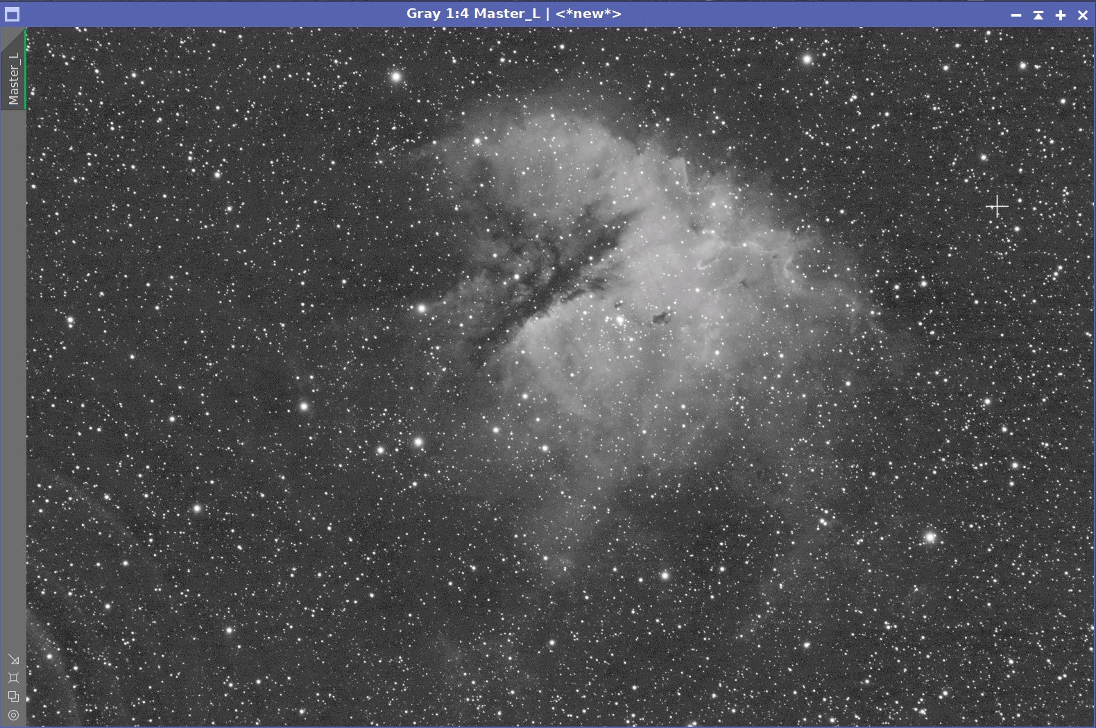
The computed Lum Image.

A 4-up panel showing the original and new computed L image for comparison.
Prepare for Deconvolution
Create PFS image using PFSImage script
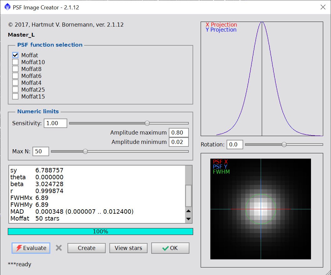
The PFSImage Panel with settings used

The resulting final PSF image
Run Starmask to create the initial LDSI image (see panel snap for parameters)

The StarMask panel set up to create the LDSI map.

The HT tool was used in this config to boost the LDSI image

Initial LDSI Image
Compare the mask to the original image - the stars in the mask are too small to cover the stars in the image.
Apply HT Boost (see panel snap for parameters)
Apply MorphologicalTransform (as seen below) as many times as necessary to cover the larger stars

Checking the LDSI image against the Master L image - Star mask images are too small. (click to enlarge)
Checking again after apply 3 more levels of boost - sizes now look good! (click to enlarge)

The Final LDSI image
Select Preview regions on the image for Decon exploration ( I failed to capture a screen snap of it for this image)
Iteratively run decon on previews until parameters are finalized (see panels snap for final values)

The final Deconvolution Parameters are shown
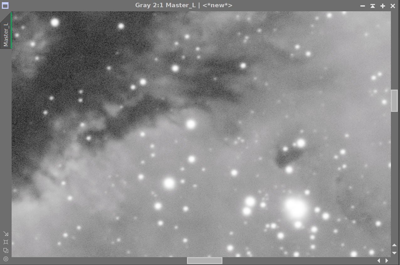
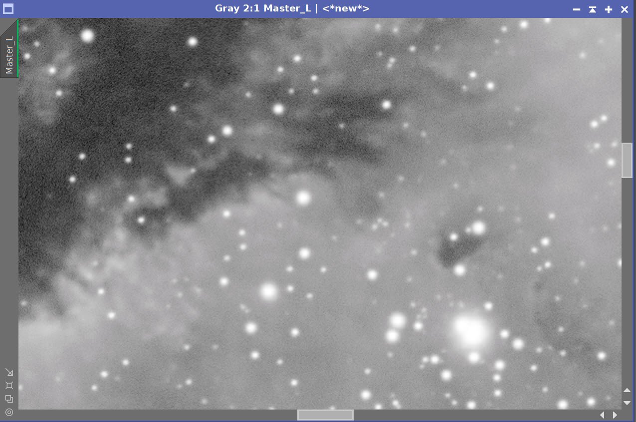
Master L - Before and After Deconvolution
Apply Noise XTerminator to the L-Image. Use a strength. of 0.6 and a detail of 0.30 to enhance detail
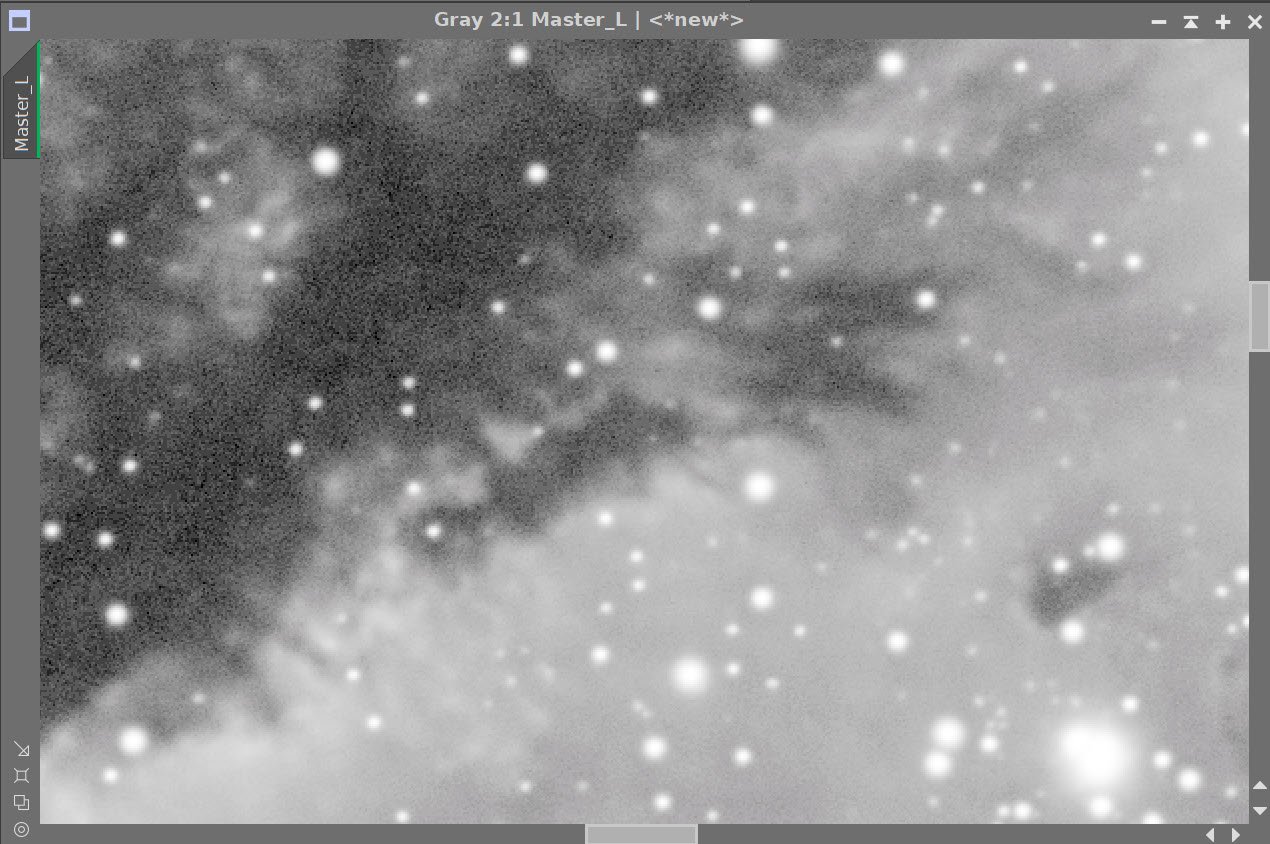
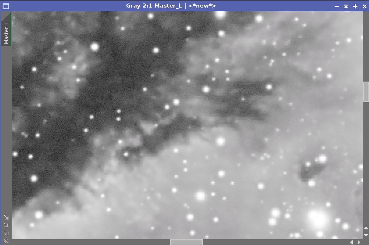
Lum image - Before and After Noise XTerminator 0.6 with Detail of 0.3
7. Process the Linear Master L Image
Take the Lum image nonlinear using the STF->HT method.
Do a final adjustment with CT. Begin to darken background to minimize the rings artifacts in the bottom left-hand corner.
The initial nonlinear L image after going nonlinear (click to enlarge)
Nonlinear L image after a CT adjustment (click to enlarge)
Create a Starless version of the image using StarXTerminator - creating a star image as well as using “Unscreen Stars”

The RC-Astro StarXTerminator Panel with settings used.
The Initial Starless L image (click to enlarge)
The initial Stars-Only Image (click to enlarge)
Note how impactful the circular ring and background noise artifacts are!
Create a Range mask
Use the RangeSelection tool to isolate the nebula
Use the Dynamic Paintbrush to remove outer artifact elements from the mask.
Apply the Rangemask and darken artifacts with CT
Create a GAME mask that uses elliptical gradients to target interesting features of the nebula
Apply the Game Mas and run LHE radius = 162, contrast limit = 2.0, Amount = 0.46, Hostogram: 8-bit
Create an initial range mask (click to enlarge)
Rang mask adjusted with the Dynamic Paintbrush (click to enlarge)
Range Mask applied (click to enlarge)
Use CT to mitigate the artifacts with the mask applied to protect the main nebula. (click to enlarge)
The Targeted GAME mask. (click to enlarge)
The Targeted Game Mask applied (click to enlarge)
L Image after LHE applied to targeted areas. (Click to enlarge)
8. Create and Process the Initial Color SHO image.
Combine Master Linear images with the ChannelCombination Tool to create the Master SHO image.
Remove stars with starXTerminator
Apply Bill Blanshan’s SHO Normalizer Script.
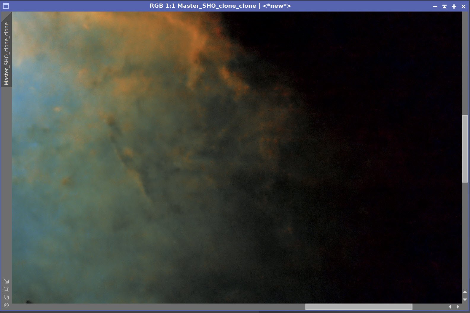
Go nonlinear with the STF->HT method
The Master SHO linear color image. (click to enlarge)
Bill Blanshan’s Normalize SHO Script. (click to enlarge)
Normalized SHO Linear Image (click to enlarge)
After Star Xterminator (Click to enlarge)
THe Symbols table for Bill Blanshan’s Normalize SHO script - showing values used. (click to enlarge)

Nonlinear SHO Image with CT adjust. (click to enlarge)
Create Color Masks
Red Nebula mask that covers the Nebula and a Red Ring Mask to cover the outer regions.
Create a red mask image using Bill Blanshan’s RedMask Script
Run Blanshan Mask Blur two times on the image
Make two copies of the mask
Use Dynamic Paintbrush to remove the outer region on one mask
Use Dynamic Paintbrush to remove the center region on the other mask
Run Blur on each mask to soften.
Create a Blue and Yellow Mask using similar methods.

Bill Blanshan’s Color Mask scripts
Initial Red Nebula Mask(click to enlarge)
Red Nebula Mask after running CT to boost. (click to enlarge)
Red Ring Mask made by removing the nebula with the Dynamic PaintBrush and blurring. (click to enlarge)
Red Nebula Mask after running Blanshan Blur twice (click to enlarge)
Final Red Nebula mask after cleanup with Dynamic Paintbrush and further blur. (click to enlarge)
Blue Mask (click to enlarge)
Yellow Mask (click to enlarge)
Blue Mask after cleanup with Dynamic PaintBrush (click to enlarge)
Yellow Mask after cleanup with Dynamic PaintBrush (click to enlarge)
Final Blue Mask after CT boost and blur (click to enlarge)
Final Yellow Mask after CT boost and blur (click to enlarge)
Apply Red Nebula Mask and Adjust with CT
Apply SCNR for Green 80%
Apply Blue Mask and adjust with CT
Apply Red Ring Mask and adjust with CT to reduce artifact visibility
Apply Yellow Mask and adjust with CT
Apply Noise XTerminator with a Strength of 0.65 and detail of 0.15
Add L-starless image in using LRGBCombination
CT adjust with Red Nebula Mask (click to enlarge)
CT Adjust with Blue Mask (click to enlarge)
CT Adjust with Yellow Mask (click to enlarge)
SCNR Green 80% (click to enlarge)
CT Adjust With the Red RIng Mask (click to enlarge)

Before and After Noise XTerminator 0.65 with detail of 0.15
Before L image Insertion (click to enlarge)
After L insertion (click to enlarge)
9. Add The Stars Back In
Apply CT to L-Stars-only image to reduce star size
Using screening Equation to Add stars back in
L-Stars-only Image (click to enlarge)
Stars-Only image after reducing tone scale with CT. (Click to Enlarge)
Screening equation to add stars back in.

Stars are now re-integrated.
10. Finish Processing the Final Image
Crop the image for better framing and composition (Note: a similar crop is necessary for any masks that you will wish to use going forward)
Apply CT to adjust the image
Run the DarkStrructureEnhance script with default terms
Run the Blanshan Star Reduction Script
Create the Starless Clone
Since we will use this to create the Star Reduced mage, I gave it a color tweak before taking the next steps
Run Version 2 with 0.25.
Apply Range Mask to protect the background
Run MLT Sharpening as documented below.
Newly Cropped Image. (click to enlarge)
CT adjust (click to enlarge)

After DarkStructureEnhancee Script (click to enlarge)

Blanshan Star Reduction Scripts
Starless Image for the Star Reduction Script (click to enlarge)
Star reduction along with a color tweak (click to enlarge)
With the Range Mask applied to protect the nebula (click to enlarge)

MLT Sharpening used.
MLT Sharped applied with mask (click to enlarge)
Final CT tweak with Blue mask in place. (click to enlarge)
11. Export to Photoshop
Save images as Tiff 16-bit unsigned and move to Photoshop
I tweaked things with the camera filter clarity, curves, and color mix - in a global adjustment
I used the lasso tool with a feather of 150 pixels and selected small areas of detail areas of the image and enhanced them with the Clarity tool.
I added watermarks and title sections
Create a High-Color and a Mid-Color version of the image
Send out for comments
The mid-Color version was preferred.
Export Clear, Watermarked, and Web-sized jpegs. as the best.
The High-Color Version (click to enlarge)
The Mid-Color and Preferred Version. (click to enlarge)
Adding the next generation ZWO ASI2600MM-Pro camera and ZWO EFW 7x36 II EFW to the platform…