
IC 1848 - The Soul Nebula - 6.8 hours in SHO (and a Change in Horses Mid-Stride!)
Date: Dec 13, 2022
Cosgrove’s Cosmos Catalog ➤#0117
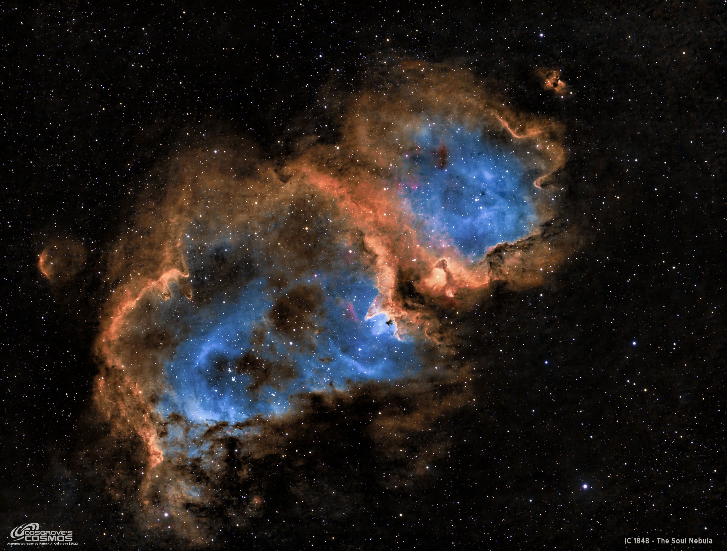
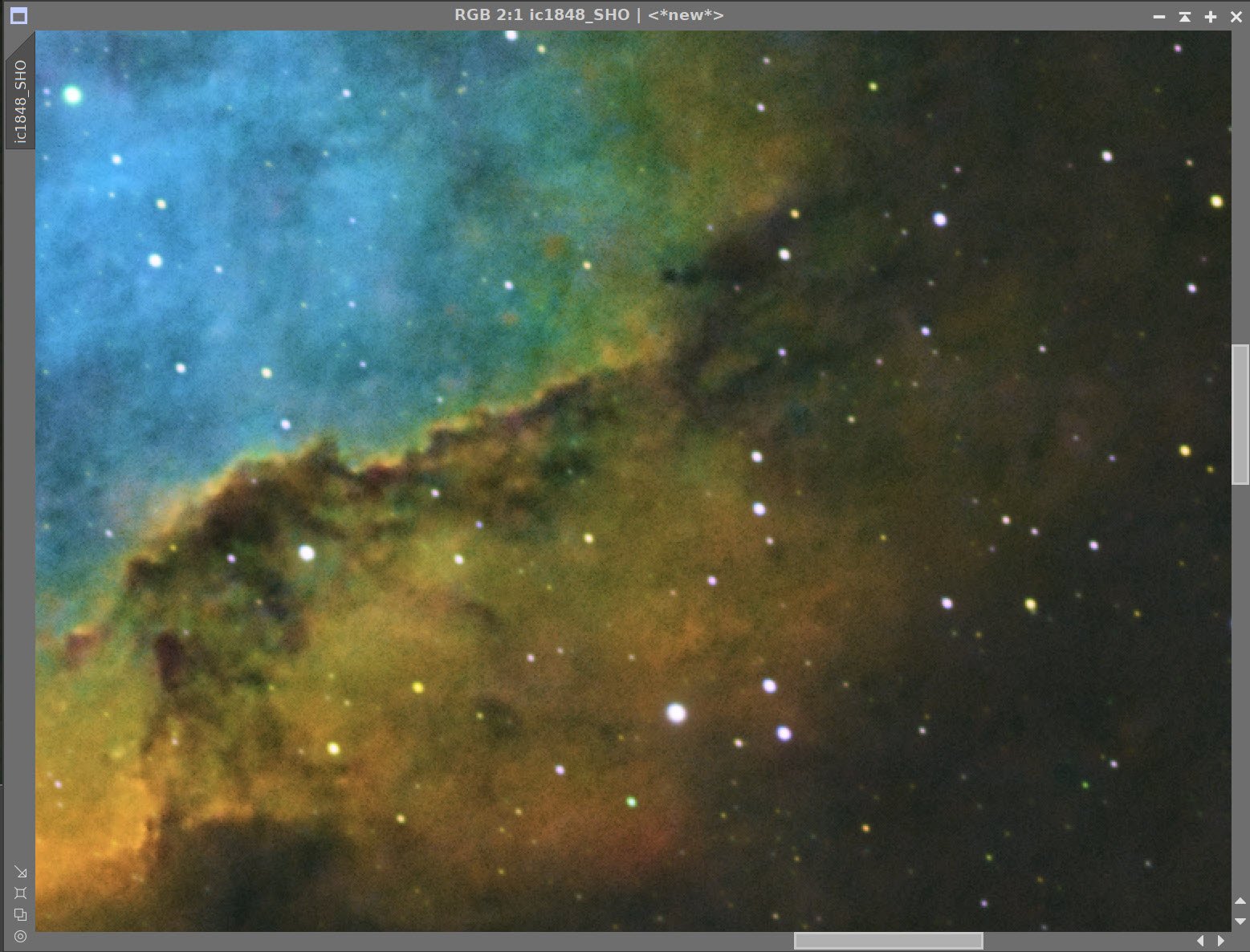
IC 1848 - The Soul Nebula - was the result of 7 hours and 40 minutes of narrowband exposure. (click for full res version via Astrobin.com)
Awarded Flickr “Explore” Status on Dec 14th!

Table of Contents Show (Click on lines to navigate)
About the Target
IC 1848, also known as “The Soul Nebula, ”The Embryo Nebula,” Sharpless 2-199, LBN 667, and Westerhout 5, is an emission nebula with an associated cluster of young hot stars located ~6,500 light-years away in the constellation of Cassiopeia. IC 1848 actually refers to an open cluster embedded in the nebula but is most often used to identify this target.
IC 205 - The Heart Nebula is close by and connected to IC 1848 (click to enlarge)
The nebula is about 100 light-years across in size.
It is often associated with the Heart Nebula (IC 1805) - another famous object which is located 2.5 degrees away in the sky.
These two regions are connected by a bridge of material and are illuminated by stars that are only about a million years old. These are mere toddlers when compared to our Sun, which is estimated to be approximately 5 billion years old.
The Annotated Image
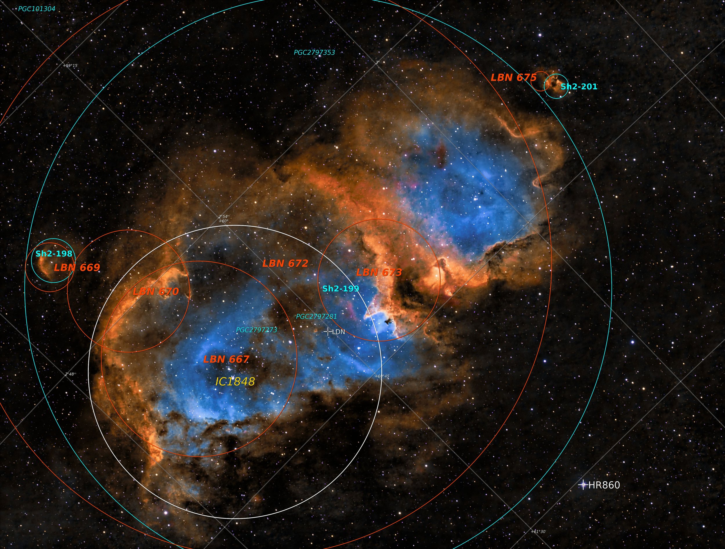
This finder chart was created with the ImageSolver and FinderChart tools in Pixinsight.
The Location in the Sky

This annotated image was created using the Pixinsight ImageSolve and ImageAnnotation scripts.
About the Project
Intro Video
A few minutes of introduction for this project by yours truly! While this project posting is quite detailed, the video allows me to discuss some aspects of the project in a more personal way.
Choosing the Target
This is the fifth and last target I have processed from my last capture session, which began in late October.
I’ve always been intrigued by the Heart and Soul Nebulae and wanted to have them in my portfolio. I shot the Heart Nebula about a year ago and was very happy with how that image came out.
I shot a small portion of the Soul Nebula using my AP130 platform. But with this scope, I could not capture the entire target - just a small portion of the “head” region. So I still wanted to come back and try with my FRA400 scope at some point.
As I looked for what targets would be well positioned for me (and my tree line) back in October, I saw that the Soul Nebula would be within reach from about 2 am until about 5:30 am.
So I added this to my shoot list - happy to be able to finally capture data on this target!
Data Capture
Most of the subs were captured over the nights of Oct 21 and 22. As documented in my previous project, I was sick with a bad cold during those nights, and things got worse to the point where we had two more beautiful clear nights that could have been used to capture more subs, but I was just too sick to care. I hate losing out on good nights!
Unfortunately, that left me in a bad state. Not only was my integration much shorter than I intended. So I held off on processing the data I had - hoping that I would get an opportunity to capture more subs.
That opportunity came a month later, on Nov 23rd. While still feeling some of the effects of my illness (it really hung in there!), I still got out and captured about another 3 hours of data for this target.
In general, these nights were clear and very cool. The first night was a bit breezy, and I was concerned about my guiding, given that my scopes are in the driveway and exposed. I did not think either night was particularly transparent - but my subs seem to be looking reasonable, and I was satisfied.
The final night was very clear and very cold. When I shut things down, I had a heavy build-up of frost on all of my equipment!
Changing Horses Mid-Ride
Typically I show the Platform an image was taken with and specify the version. The version is important because, over time, I have evolved the configuration of each platform. Each version is documented and shown as part of the image project posting.
This project will be a little odd in that respect. The first two nights were captured with version 1.5 of my Askar FRA400 Astrograph setup, using the IOptron CEM26 mount. The third night, however, was done with a completely different mount!
By this time, I had swapped over to the new ZWO AM5 Harmonic mount!
Since most of this project was done with the old configuration, I will use version 1.5 as the main entry. Another reason is that I have not yet created the posting for version 2.0 with the new config! This will take some time as I want to document why I made the change and what this change entailed.

For the first two nights, the data was captured with this configuration using the IOPtron CEM26 mount.

For the last night, I had swapped over to my new mount - the ZWO AM5 Harmonic drive!
Why the change? That will be covered in the ver. 2.0 posting, but I will share a few key points here:
When I first got the CEM26 - it was clearly the best mount for the price if you wanted a lightweight, portable mount with a decent load capacity for the weight of the mount itself.
It has performed really well for me but
I keep needing to adjust the DEC belt tension to reduce DEC backlash - then it still slips.
I have been getting more slop in the guiding, and it seems like something has loosened up in the drive. This is something I need to resolve.
The AM5 is the new kid on the block, and I was interested in a Harmonic drive as it offered:
An even better weight to the load-bearing specification as no counterweight was needed!
No need to precisely balance the load
It seemed to be a quality mount - but it was much more expensive.
But how would it perform?
So the third night would be my very first time using that mount, and I was still learning how to use it. I had to change my hardware configuration, and I had to set up the software to work with this new arrangement.
After calibrating PHD2 with the new mount, I also ran Guide Assistant to tune the parameters a bit.
I ran into another problem that evening with my camera. The SGP controls did not seem to be able to control the cooler on the camera. I tried reinstalling ASCOM drivers and SGP itself, but I could not get the controls to go active. Left alone, the camera seemed to be cooling to -10C. So I decided to go ahead with this temp and collected not only light frames for the night but a full set of calibration files as well. (This is another thing I will need to straighten out!)
As it turned out, the AM5 did an amazing job! With the CEM26, I was ecstatic when I could get RMS guide errors of less than 1.60. Some nights, I got it as low as ~ 1.0. Given the 400mm focal length - even 1.6 did pretty well.
With the first evening of use, I was getting RMS errors 0f 0.38! This is the lowest guide error I had ever measured!

Here is the CEM26 PHD2 guide log for the night of October 22. I was getting some elongated stars. The guide RMS guide error for this segment was 1.13 - very good for this mount!

Here is my PHD2 guide log for the night of Nov 23 using the AM5. The vertical scale is about the same - you can see that the AM5 is doing a lot better- RMS errors of 0.35 for this segment!
Data Analysis
Blink analysis showed that the data looked pretty solid for all filters. A few frames needed to be removed. I ended up with just a bit over 7.8 hours of narrowband data.
But I did see something disturbing as well.
Many frames from the CEM26 mount had elongated stars. Not so much on the Ha frames as the O3 and S2 frames.
The frames from the AM5 have nice tight and round stars in all instances.
So the question was - how was I going to deal with this?
Normally I would throw out those frames that had problems like this - but I was so short on integration time I really did not want to do that.
So I figured I had two options:
I could hope that rejection would clean things up a bit
Since I was going to be doing starless processing, if push came to shove, I could use the image of the stars from just the AM5 mount for this purpose. I would have to see how things worked out, but I was feeling fairly optimistic about my ability to deal with this problem in the data.
Previous Efforts
As I indicated, I have shot this target once in the past - back in December of 2021. This was some data from an aborted run. I only had one clear evening and only had 2 hours of integration. It was taken on my AP130 platform, so I could only frame a small portion of the nebula - covering a portion of the head. Despite the low integration, I tried processing my data and was surprised to get a reasonable image out of it.
You can see that project posting HERE. You can see that image below - along with the current one, for comparison.
IC 1848 - taken in Dec 2021 (click to enlarge)
IC 1848 - our current image (click to enlarge)
Image Processing
This project, just like the last few, is an SHO narrowband capture with 5-minute subs. It follows my standard workflow for these kinds of images - as updated when using the SHO Normalization Script by Bill Blanshan.

The processing flow for this project.
A Change in Workflow
In my normal workflow, I take the Master Ha, O3, and S2 images nonlinear, tweak them one-to-another, and then combine them to create a nonlinear SHO image. This image must then be adjusted to deal with the strong green colors you get when strong Ha images are mapped to the Green channel in the SHO mapping. This workflow has worked very well for me.
However, I saw that Bill Blandshan has created some new Pixelmath Scripts that manage the normalization of SHO images, and I wanted to try this out.
To use this script, you combine the linear master images into a linear SHO color image. You then take this image starless and apply his script. As with most of his scripts, there are a few parameters that you can adjust to change how the script operates. But with one button push, you have a normalized SHO image. This sounded very attractive.
So for this project, I adopted this change in workflow. The results were quite good.
High Color vs. Mid-Color Results
When it comes to astrophotography, I am a high-color guy. However, my natural inclinations tend to create images with perhaps too much saturation. Every time I have tested this with a high-color version vs. a low-color version, the feedback always sides with the lower-color position.
I think that rather than constantly asking for feedback and getting the same answer, it would be better if I processed the image the way I normally would and then back off a bit on the color saturation.
See the two offerings below:
Here was my High-Color Version. (click to enlarge)
And here is my Mid-Color version of the image. (click to enlarge)
I still like the snap and pop I get with the bolder colors, but I will put the mid-color version forward as my image.
Results
In general, I am very pleased with the image as it came out. My only complaint is that I ended up with low integration, and this has caused some of the very faint nebulosity in the background sky to be a little patchy or mottled. In fact, I saw some of this in some of the darker areas of the main nebula. Doubling the integration would have given me a smoother and cleaner data set.
A detailed Processing Walk-Through is provided for this image at the end of the posting…
More Information
Wikipedia: Soul Nebula
Constellation-Guide.com: Soul Nebula
The Sky-Live: Soul Nebula
Capture Details
Lights Frames
Data were collected over two nights: Oct 21 & 22 and Nov 23.
34 x 300 seconds, bin 1x1 @ -15C, Unity Gain, Astronmiks 6nm Ha
24 x 300 seconds, bin 1x1 @ -15C, Unity Gain, Astronmiks 6nm O3
24 x 300 seconds, bin 1x1 @ -15C, Unity Gain, Astronmiks 6nm S2
Total of 6 hours 50 minutes
Cal Frames
25 Darks at 300 seconds, bin 1x1, -15C, Unity Gain
15 Flats at bin 1x1, -15C, Unity Gain - for Ha, O3, & S2 filters
25 Dark Flats at Flat exposure times, bin 1x1, -15C, Unity Gain
Software
Capture Software: PHD2 Guider, Sequence Generator Pro controller
Image Processing: Pixinsight, Photoshop - assisted by Coffee, extensive processing indecision and second-guessing, editor regret, and much swearing…..
Capture Hardware:
Scope: Askar FRA400 f/5. 6 Astrograph
Focus Motor: ZWO EAF 5V
Guide Scope: William Optics 50mm guide scope
Guide Scope Rings: William Optics 50mm slide-base Clamping Ring Set
Mount: IOptron CEM 26 for ist 2 nights
ZWO AM5 for 3rd night
Tripod: Ioptron 1.5” Tripod
Camera: ZWO ASI1600MM-Pro
Camera Rotator: Pegasus Astro Falcon Camera Rotator - new
Filter Wheel: ZWO EFW 1.2 5x8
Filters: ZWO 1.25” LRGB Gen II, Astronomiks 6mm Ha, OIII,SII
Guide Camera: ZWO ASI290MM-Mini
Dew Strips: Dew-Not Heater strips for Main and Guide Scopes
Power Dist: Pegasus Astro Powerbox Advanced
USB Dist: Pegasus Astro Powerbox Advanced
Polar Alignment
Cam: Iplolar
Software:
Capture Software: PHD2 Guider, Sequence Generator Pro controller
Image Processing: Pixinsight, Photoshop - assisted by Coffee, extensive processing indecision and second-guessing, editor regret, and much swearing…..
Click below to see the Telescope Platform version used for this image:
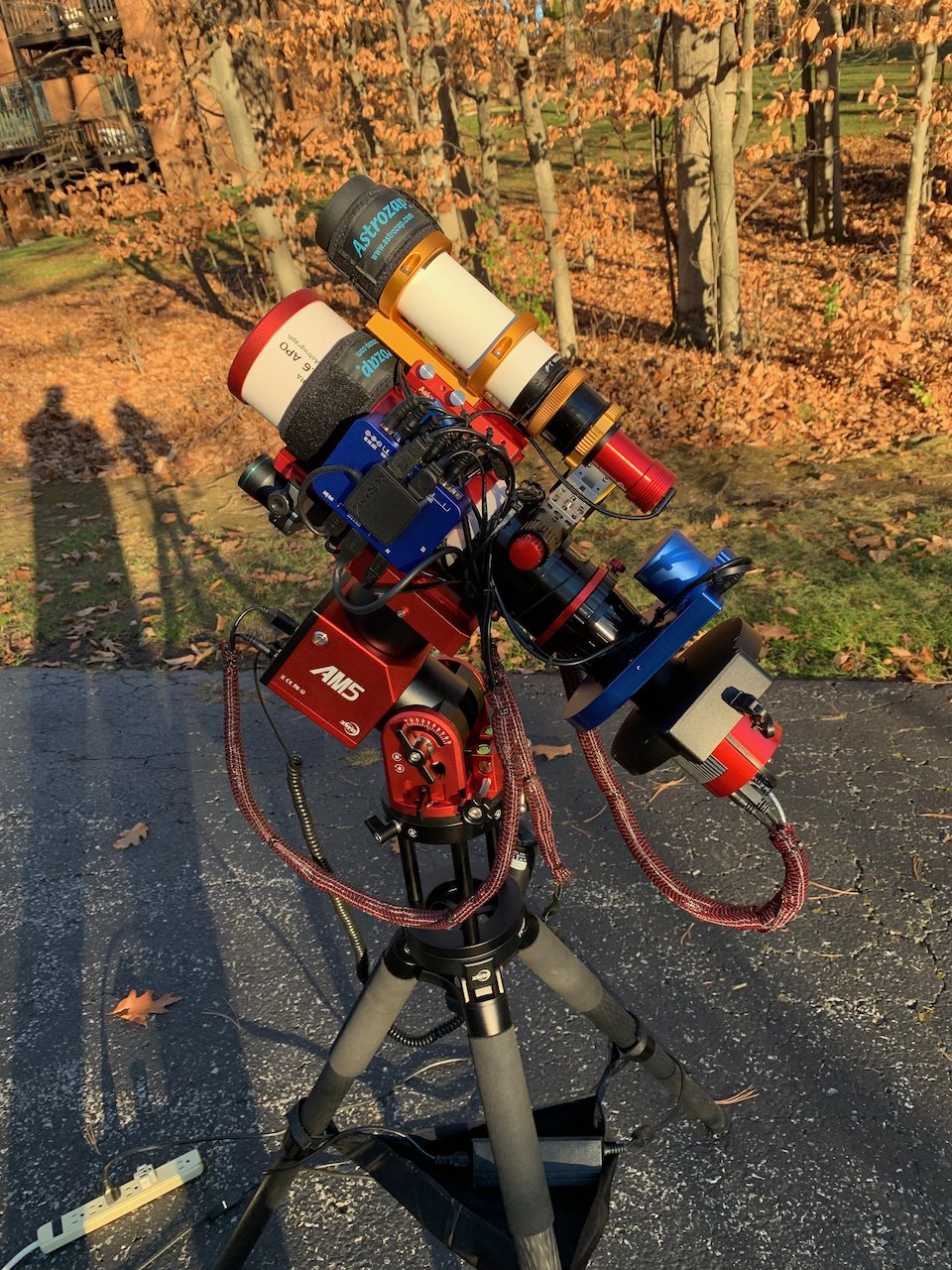
The updated platform with the ZWO AM5.
Image Processing Walk-Through
(All Processing is done in Pixinsight - with some final touches done in Photoshop)
1. Blink Screening Process
Ha
2 frames showed no nebula - deleted
Others looked good
The second night showed elongated stars
O3
One frame had a tracking issue - removed
Some gradients
Some egg-shaped stars on the CEM26 mount - not seen on AM5
S2
Again CEM26 has egg-shaped stars, and AM5 does not
AM5 exposure seems to be less exposed - thin clouds?
Nothing removed
Flats
Some variance was seen in brightness on night 3 - is the cold causing variance on LED panel?
4 outliers were removed because of this
Darks
From sh2-129 project
300-second darks all looked good.
Dark Flats
looks good.
I am not sure why I am suddenly seeing more variations in the flats. It was very cold, and I wonder if the panel I am using gets a little strange in the cold. In the future, I will increase my sample size for flats on cold nights.
2. WBPP 2.5.4
Reset all
Load all lights
Load all flats
Loads darks from sh2-129 project
Select peak quality
Keyword “Night”
Ref image - auto
Output folder wbpp
Set Darks exposure threshold to 0
Set Lights exposure threshold to 0
Disable astrometric solution (Dynamic Crop destroys it anyways!)
Map missing flats
Map missing dark flats
Set the Pedastal image to auto for all filters
Set cosmetic correction or all frames
Executed in 18:04 minutes - no errors

WBPP Calibration View

WBPP Post Calibration View
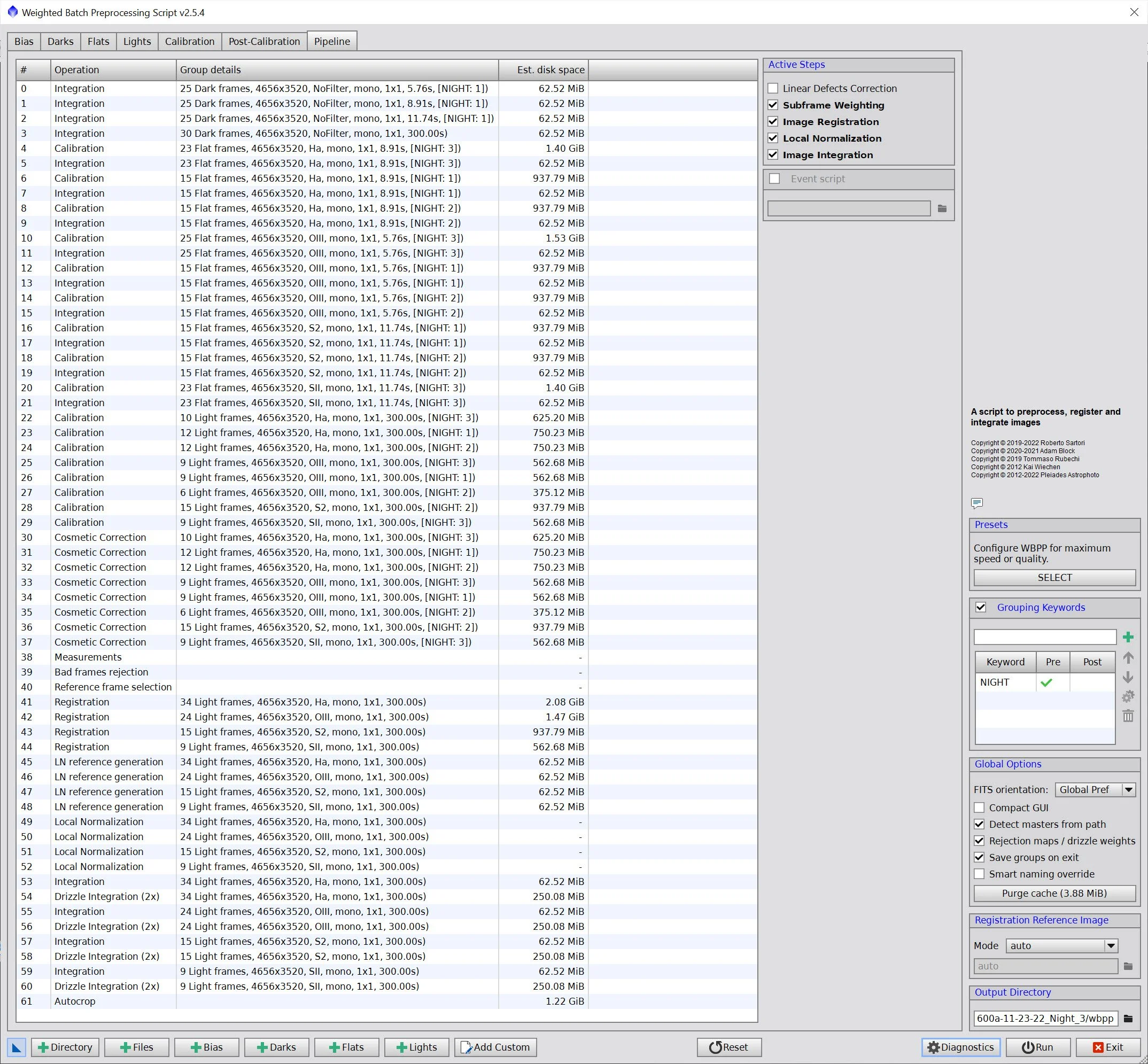
WBPP Pipeline View
3. Run Image Integration for all Master Images
Use ImageIntegration to create master images and collect rejection maps
Apply a Dynamic Crop to all three master images to clean up the edges.
Note that at this point - we still have elongated stars. Rejection seemed to reduce this - but they are still there. However, we will remove stars - we will have to ensure that the ones we add back in are not elongated.
I ran SubframeSelector and checked for Eccentricity - clearly, you can see that the eccentricity of the stars is high for the first two nights and is reduced for the last night.

ImageIntegration Panel with setup used to create Master Images.
Rejection High - Ha (click to enlarge)
Rejection Low - Ha (click to enlarge)
Rejection High - O3 (click to enlarge)
Rejection Low - O3 (click to enlarge)
Rejection High - S2 (click to enlarge)
Rejection Low - S2 (click to enlarge)
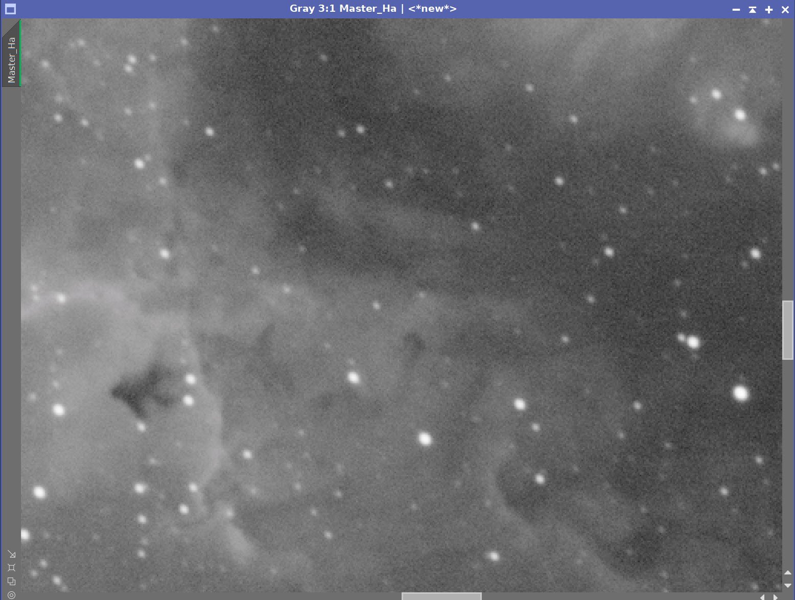
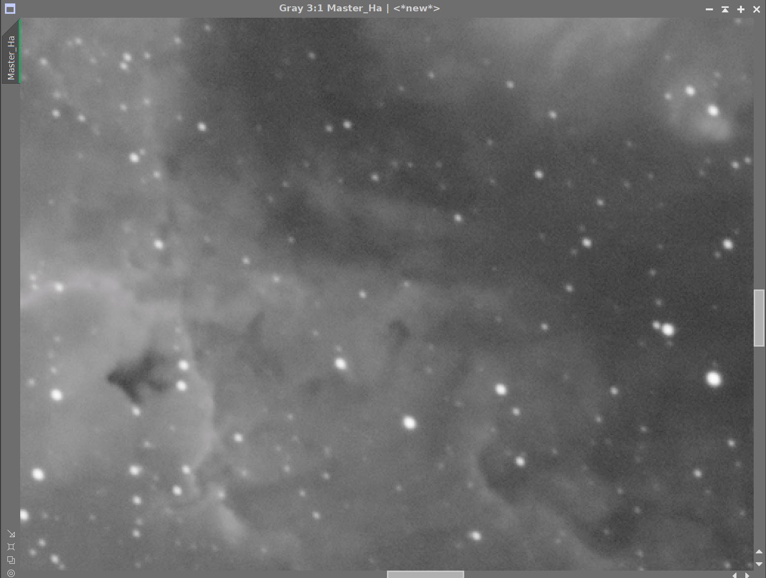
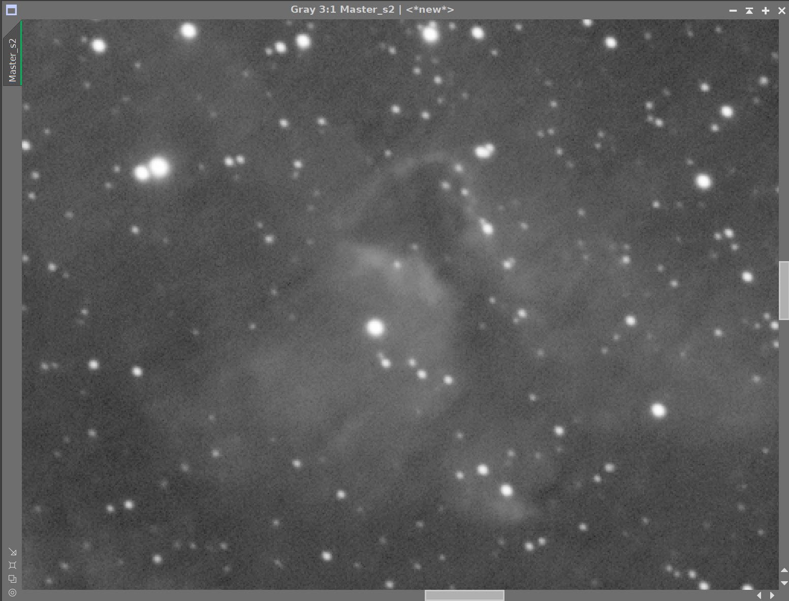
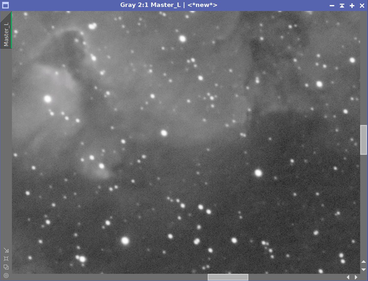
Master Ha (click to enlarge)
Master O3 (click to enlarge)
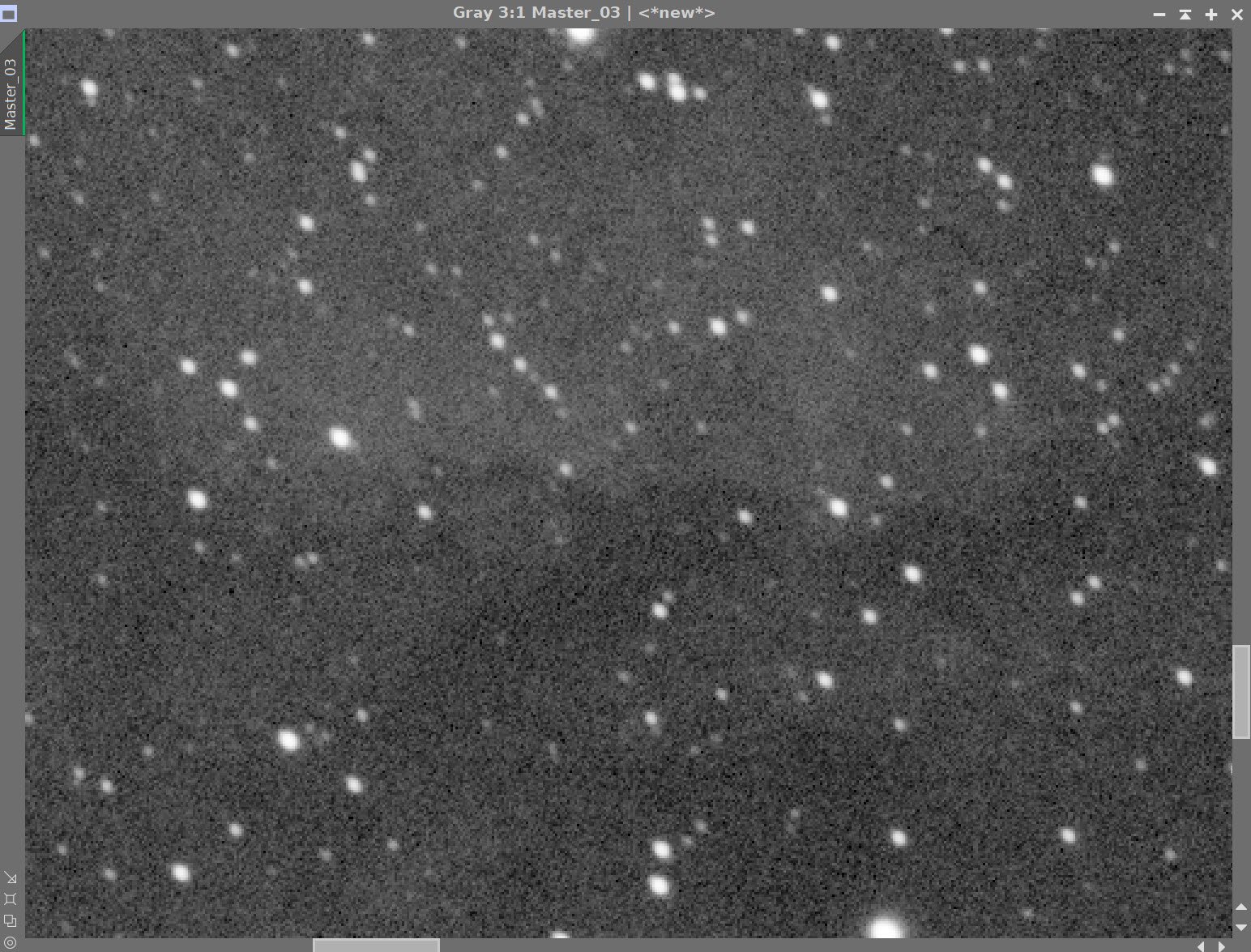
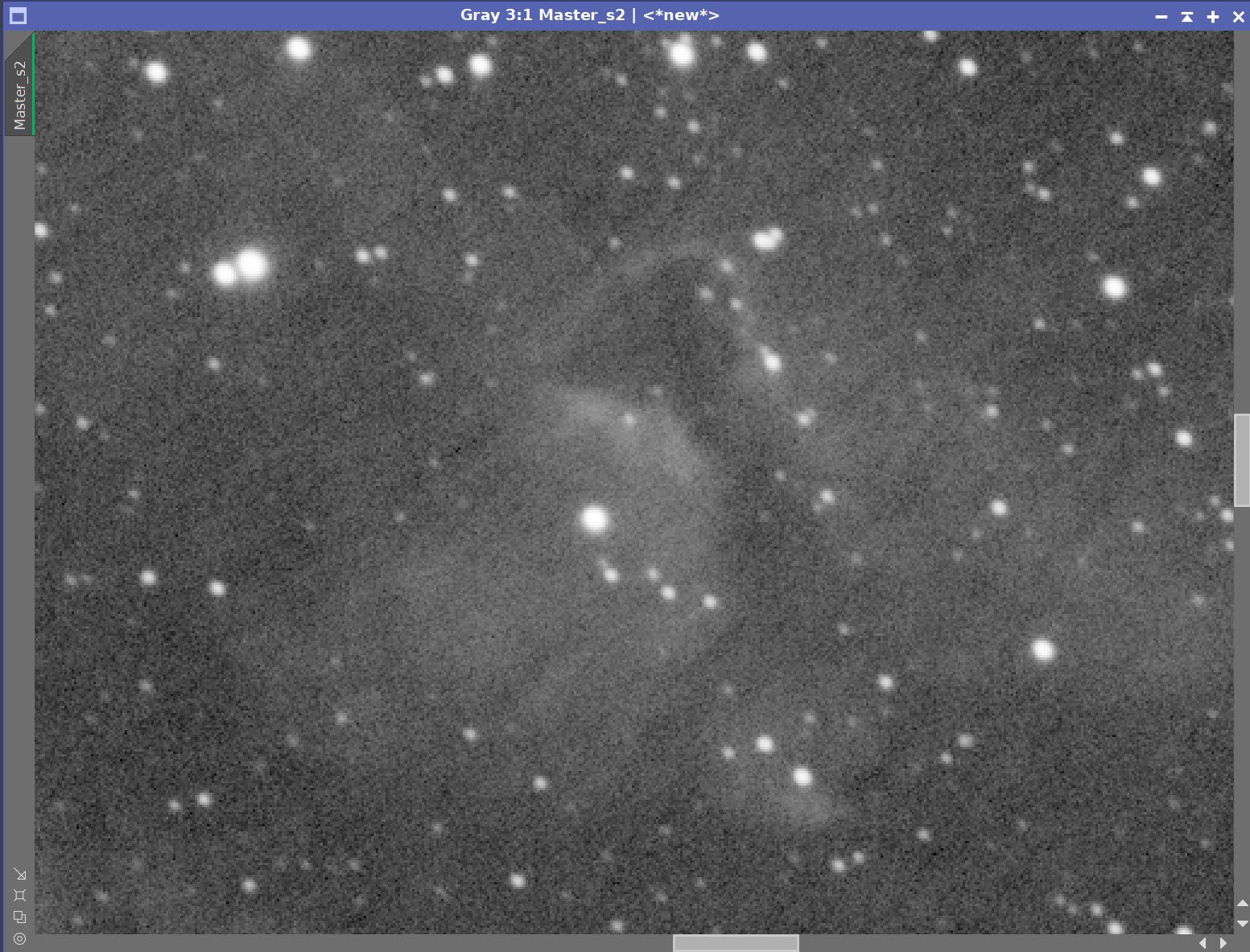
Master S2 (click to enlarge)
Ha Eccentricity plot. Note reduced Ecc at the end of the plot. (click to enlarge)
O3 Eccentricity plot. Note reduced Ecc at the end of the plot. (click to enlarge)
S2 Eccentricity plot. Note reduced Ecc at the end of the plot. (click to enlarge)
4. Dynamic Background Extraction
DBE applied to all images
DBE Sampling for Ha (click to enlarge)
DBE Sampling for O3 (click to enlarge)
DBE Sampling for S2 (click to enlarge)
Ha - Before DBE (click to enlarge).
O3 - Before DBE (click to enlarge).
S2 - Before DBE (click to enlarge)
Ha - After DBE applied (click to enlarge).
O3 - After DBE applied (click to enlarge)
S2 - After DBE (click to enlarge)
Ha - Background extracted (click to enlarge)
O3 - Background extracted (click to enlarge)
S2 - Background extracted (click to enlarge)
5. Apply light Noise Reduction to the Ha, O3, and S2 Linear Master Images
Ha: Apply Noise XTerminator with a value of 0.5, detail of 0.20
O3: Apply Noise XTerminator with a value of 0.7, detail of 0.20
S2: Apply Noise XTerminator with a value of 0.6, detail of 0.20

Master Linear Images - Before and After Noise XTerminator
7. Create the Synthetic Lum image and Finish The Linear Processing of It
We have three master images, which means we can use ImageIntegration to create the Synthetic Luminance Image.
I saved the three master images to disk.
I set up ImageIntegration to use those files, averaging for integration and disabling rejection.
Run and rename the new resulting Luminance image.

ImageIntegration Panel as used to create the Synthetic Lum image.

The weights computed by ImageIntegration to combine the images

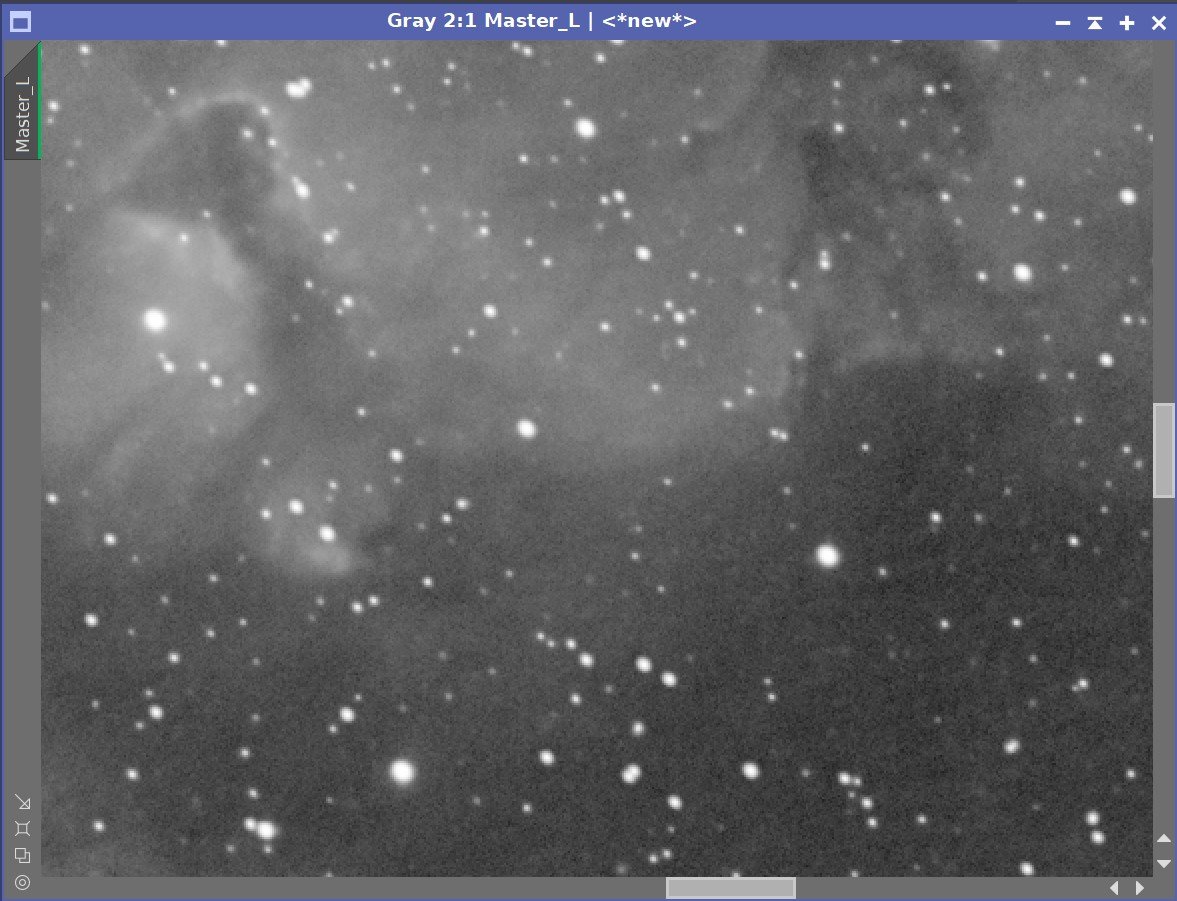
The computed Lum Image.

A 4-up panel showing the original and new computed L image for comparison.
Prepare for Deconvolution
Note - I did not drizzle process this image, and because the FRA400/ASI1600MM-Pro combination is slightly undersampled, I don’t expect that we will get great results from deconvolution, but I am going to try and see what I can do.
Create PFS image using PFSImage script
Note that the PFS model is a little square and blocky.

The PFSImage Panel with settings used (note blocky PFS!)

The resulting final PSF image
Run Starmask to create the initial LDSI image (see panel snap for parameters)

The StarMask panel set up to create the LDSI map.

The HT tool was used in this config to boost the LDSI image

Initial LDSI Image
Compare the mask to the original image - the stars in the mask are too small to cover the stars in the image.
Apply HT Boost (see panel snap for parameters)
Apply MorphologicalTransform (as seen below) as many times as necessary to cover the larger stars

Checking the LDSI image against the Master L image - Star mask images are slightly too small. (click to enlarge)
Checking again after apply 3 more levels of boost - sizes now look good! (click to enlarge)

The Final LDSI image
Select Preview regions on the image for Decon exploration
Iteratively run Decon on previews until parameters are finalized (see panels snap for final values)


The final Deconvolution Parameters are shown
Master L - Before and After Deconvolution
8. Process the Linear Master L Image
Take the Lum image nonlinear using the STF->HT method.
The initial nonlinear L image after going nonlinear (click to enlarge)
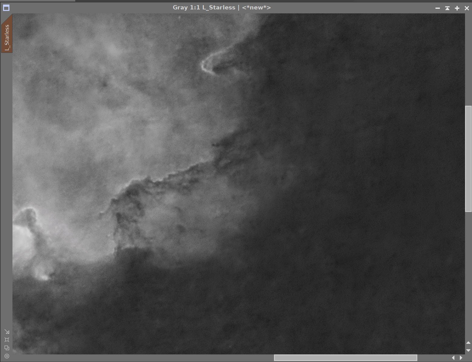
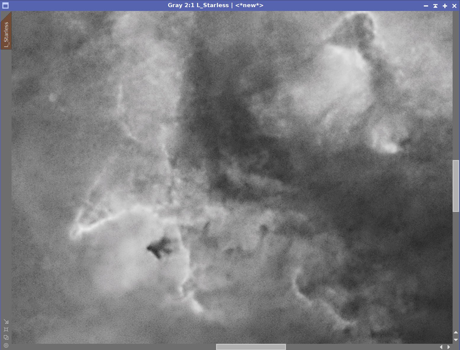
Create a Starless version of the image using StarXTerminator - creating a star image as well as using “Unscreen Stars”
Apply HT and adjust left side of the histogram
Apply CT and adjust tone scale

The RC-Astro StarXTerminator Panel with settings used.
The Initial Starless L image (click to enlarge)
The initial Stars-Only Image (click to enlarge)
HT Adjust (click to enlarge)
CT Adjust (click to enlarge)
Create a Subject Mask
Make a copy of the image
Use HT to adjust the extremes to isolate the nebula
Soften with Convolution
Apply the Subject mask and Invert to target the background
Run Noise XTerminator with a strength of 0.65 and a detail of 0.2
Create an initial Lum mask (click to enlarge)
Lum mask adjusted with HT (click to enlarge)
Soften with Convolution. (click to enlarge)
Subject Mask applied and Inverted. Now we can target the background (click to enlarge)
With Subject Mask Applied and Inverted: Before and After Noise XTerminator 0.65/0.2
Invert the Subject Mask again to target high-signal areas
Apply LHE with a radius of 64, contrast limit of 2.0, amount of 0.2, and an 8-bit histogram
Apply LHE with a radius of 300, contrast limit of 2.0, amount of 0.2, and a 10-bit histogram
Apply MLT sharpening - see panel snap below.
Subject Mask inverted again - targeting high signal areas. (click to enlarge)
Apply LHE (click to enlarge)
L Image after second LHE applied to targeted areas. (Click to enlarge)

Sharpening used with Subject Mask

Before and After MLT Sharpening with Subject Mask
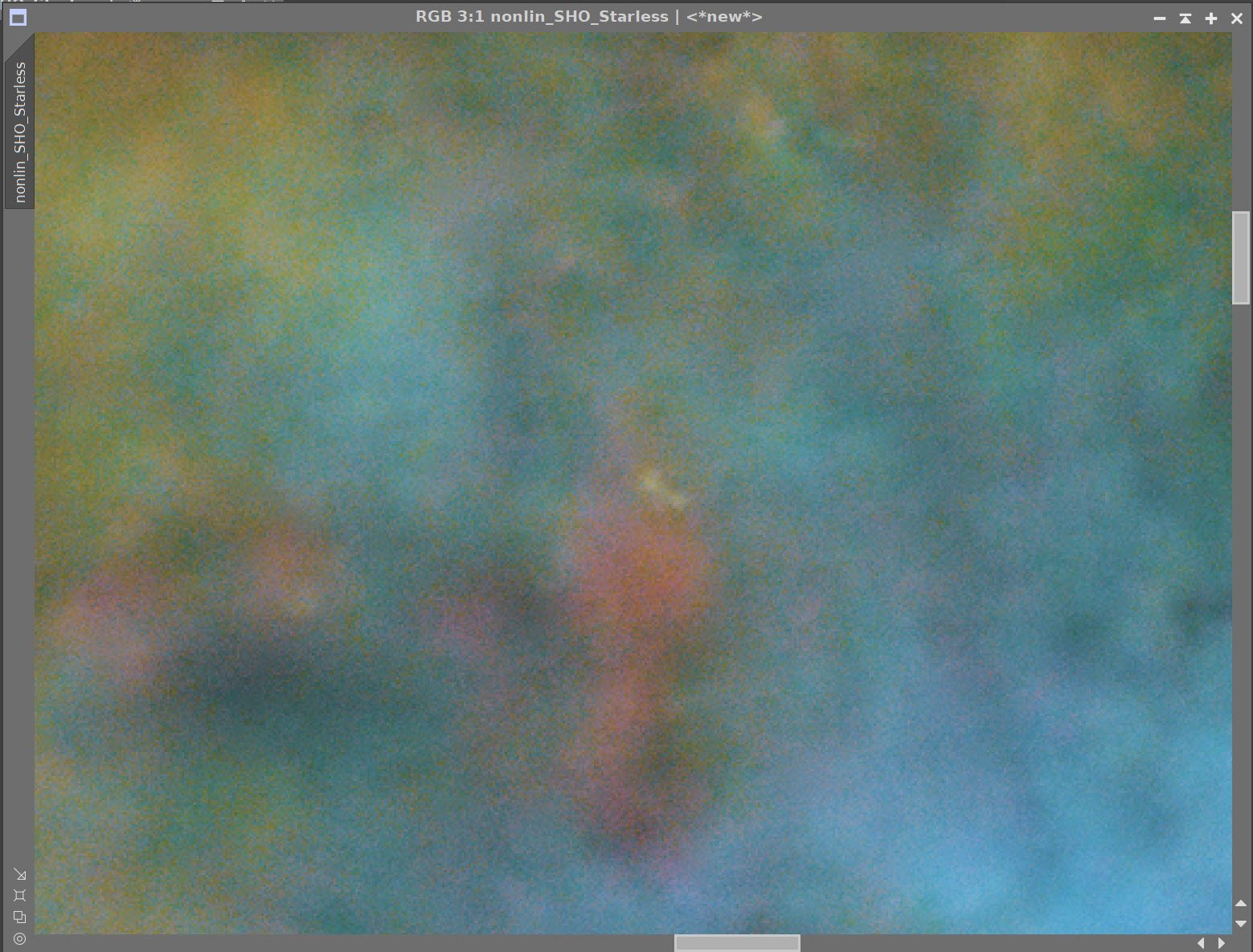
8. Create and Process the Initial Color SHO image.
Combine Master Linear images with the ChannelCombination Tool to create the Master SHO image.
Remove stars with starXTerminator
Apply DBE
Apply Bill Blanshan’s SHO Normalizer Script.
Go nonlinear with the STF->HT method
Apply CT an adjust tone scale.
The Master SHO linear color image. (click to enlarge)
Master SHO DBE Sampling (click to enlarge)
Master SHO DBE Before (click to enlarge)
Master SHO - After DBE (click to enlarge)
Master SHO DBE Background (click to enlarge)


Default Terms used with Bill Blanshan’s SHO Normalization Script
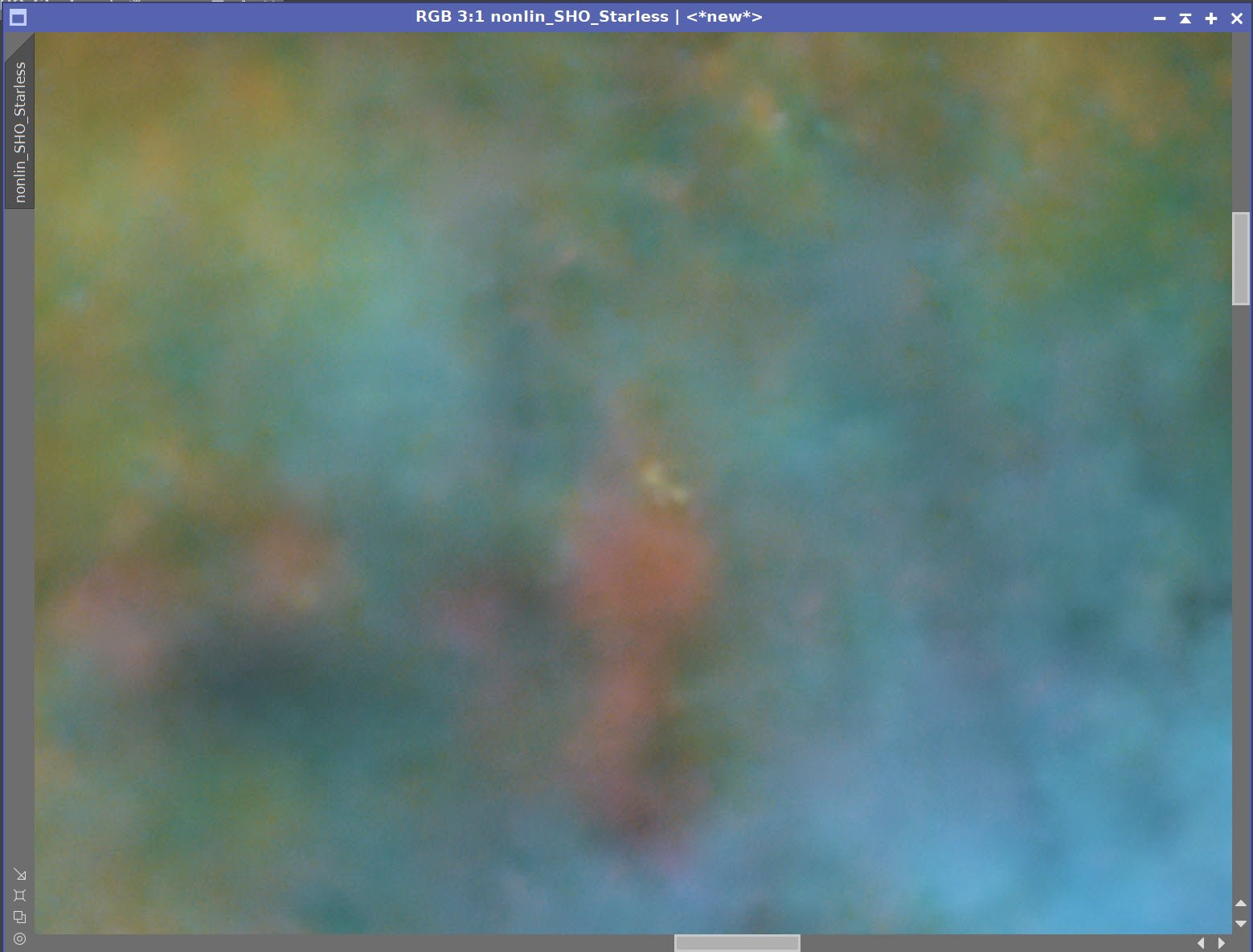
After SHO Normalization (Click to enlarge)
Gio nonlinear and apply CT(click to enlarge)
Apply the Subject mask and invert it so that the background is the focus.
SCNR Blue with 80% to remove blue in the background sky
There is a lot of magenta noise in the background. To address this:
Remove the mask
Invert the Image
Apply the Subject Mask and invert to target the background
Use SCNR green 80%
Remove the mask
Invert the image again
Add the Subject Mask Back in and Invert it.
Run SCNR Red 80%
Remove the Mask, run CT to adjust the global tone scale
At this point, I think the image still looks too green for me, so I ran SCNR Green 50% to pull this back a bit. I was happy with this and ready to start some advanced tweaking of color using masks. But first, we need to make some color masks up.
Apply Subject mask and Invert, SCNR Blue 80%. (Click to enlarge)
Apply SCNR Green 80% (click to enlarge)
Remove mask, and run CT and Adjust the global tone scale (click to enlarge)
Remove the Mask and invert the image. THis makes the Magenta noise in the background Green. (Click to enlarge)

Add subject mask back in and invert it,. SCNR Red 80% (click to enlarge)
Still a bit too green for me. Run SCNR Green 50% (click to enlarge)
Create Color Masks using the Bill Blanshan Color Maks Scripts
Create Blue mask
Create a Blue mask image using Bill Blanshan’s BlueMask Script
Boost the image with HT
Blur the mask with one or more applications of Bill Blanshan’s Blur Script.
Repeat for Yellow, Red, Cyan, and Green

Bill Blanshan’s Color Mask scripts
Initial Blue Nebula Mask(click to enlarge)
Initial Yellow Mask (click to enlarge)
Red Mask (Click to enlarge)
Cyan Mask (click to enlarge)
Green Mask (click to enlarge)
Blue Mask Blur (click to enlarge)
Yellow Mask boost (click to enlarge)
Red Mask initial Boost (click to enlarge)
Cyan Mask Boost (click to enlarge)
Green Mask Boost (click to enlarge)
Blue Nebula Boosted(click to enlarge)
Yellow Mask Blurred (click to enlarge)
Red Mask Boost and Blur (click to enlarge)
Cyan Mask Blur (click to enlarge)
Green Mask Blur (click to enlarge)
Apply the Blue mask and adjust it with CT
Apply the Green mask and adjust it with CT
Apply the Yellow mask and adjust it with CT
Apply the Cyan mask and adjust it with CT
Apply the Red mask and adjust it with CT
Apply Noise XTerminator with strength 0.7 and detail 0.15
Apply the Blue Mask and apply CT (click to enlarge)
Apply the Yellow mask and adjust with CT (click to enlarge)
Apply the Green Mask and adjust CT (click to enlarge)
Apply the Cyan Mask and adjust CT (click to enlarge)

Apply the Red Mask and adjust CT (click to enlarge)
Before and After NoiseXTerminator - strength 0.5, detail 0.15
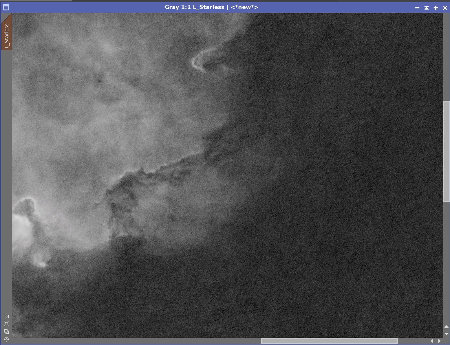
Add the L_Starless image using LRGBCombination Tool.

L_Starless Image injected.
9. Add The Stars Back In
I could use the L-Stars-only or the Nonlin_SHO_Stars_only Image for stars. I decided to try the SHO version to get some color in if I could. The quality of the stars looks pretty good, with no hint of egg-shaped stars.
Apply CT to SHO-Stars-only image to reduce star size
Using screening Equation to Add stars back in - see screen below
SHO Stars-only Image (click to enlarge)
Stars-Only image after reducing tone scale with CT. (Click to Enlarge)
Zoomed in on the stars: Pretty round and well formed - with just a hint of color. (click to enlarge)
Screening equation to add stars back in.

Stars are now re-integrated.
10. Finish Processing the Final Image
Apply CT to the image to tweak the tone scale, not that the stars are back in
Run the DarkStrructureEnhance script with default terms
Run the Blanshan Star Reduction Script
Create the Starless Clone
Since we will use this to create the Star Reduced mage, I gave it a color tweak before taking the next steps
Run Version 2 with 0.35.
Problem found with my Monitor Calibration - I resolved that and found I thought things looked too green. So I did a couple of things to fix it:
SCNR Green 20%
CT with a color curve adjustment.
Newly Cropped Image. (click to enlarge)
DarkStructureEhnance Script(click to enlarge)

Blanshan Star Reduction Scripts
Starless Image for the Star Reduction Script (click to enlarge)
Star reduction using Bill Blanshans Method 2 at 0.35 (click to enlarge)

Before and After Noise XTerminator - Strength 0.5, detail 0.2
SCNR Green 20% (click to enlarge)
Final CT after Screen Calibration Issue solved. (click to enlarge)
11. Export to Photoshop
Save images as Tiff 16-bit unsigned and move to Photoshop
I tweaked things with the camera filter clarity, curves, and color mix - in a global adjustment
I used the lasso tool with a feather of 150 pixels and selected small areas of detail areas of the image and enhanced them with the Clarity tool.

I added watermarks and title sections
Create a High-Color and a Mid-Color version of the image
I decided to lead with the mid-Color version
Export Clear, Watermarked, and Web-sized jpegs.
The High-Color Version (click to enlarge)
The Mid-Color and Preferred Version. (click to enlarge)
After doing manual camera rotations to achieve the compositional framing that I plan - using SGP’s Framing and Mosaic Wizard - I finally decided to add a Camera Rotator to this rig to automate the rotation between objects and when getting flat cal frames for images shot with a specific camera rotation. While I had the rig apart, I re-tensioned the declination belt on the mount to reduce declination backlash.