
Deconvolution in Pixinsight - Part 7: Example - Messier 31
March 26, 2022

This posting is part of seven-part series: "Using Deconvolution in Pixinsight."
Navigate to other parts of this Series:
Table of Contents Show (Click on lines to navigate)
Messier 31 in LHaRGB
This version of Messier 31 was the result of about 6 hours of integration in LHaRGB, taken with my Askar FRA400 72mm Astrograph, a ZWO ASI1600MM-Pro camera with Astronomiks filters, and an IOptron CEM60 mount.
The story of this image can be seen HERE.
This is a fairly wide field scope and the expectation is that there will not be many benefits to be had from applying Deconvolution to this image.
In addition, This telescope configuration tends to undersample the image a bit. Given the focal length and the undersampling, I did not have high hopes for Deconvolution. So I decided to drizzle-process the image to get double the resolution. I thought the drizzle processing would make this an interesting test case. I applied deconvolution to the L layer and integrated that with the RGB image using LRGBCombination. Let’s see how this worked out.

Preparing for Deconvolution
Creating The Object Mask
This was done starting with a copy of the L image, taking it nonlinear with the STF->HT method. I then used HT to clip the blacks and saturate the signal areas. Finally, I applied a bit of convolution. This gave me the following:

The M31 Object Mask.
Creating the LDSI Image
Next, I created a Local Deringing Support Image using the methods described in the previous example. Because of the high resolution of this image, I did increase the scale up to 8 to include larger stars. Given the sheer number of stars in this field, le LDSI support image came out as a pretty busy field:

M31 LDSI image. Ignore the arrow - I failed to move the cursor when I did the screen shot!
Creating the PSF Image
Finally, I used the PSFImage script to create my PSF image. Because of the drizzle processing and the high-resolution nature of the file, I changed the default Max N parameter from 50 to 150 (well - 149 actually ;-))

This is the PSFImage panel after I computed my PSF image.

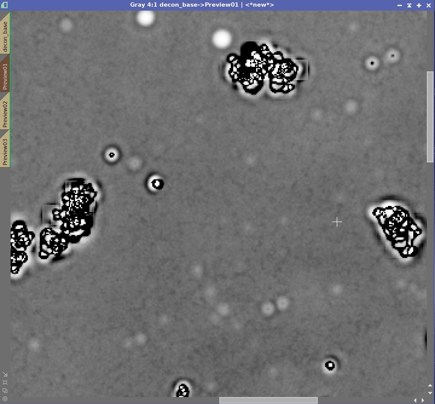
When you look at the star map that PFSImage produces, showing what stars it selected, it looked like NO stars were outlined in magenta. But if you zoom in, you can see them. There were just SO many stars in this image that PSFImage selected what is needed to compute the results. You can see in this zoomed-in view, that the stars selected were mid-range well behaved stars!

This is the final PSF Image. Note how smooth and large it is. Drizzle processing seems to have taken us from the realm of undersampling and to the realm of oversampling!
Setting Things Up to Run Deconvolution
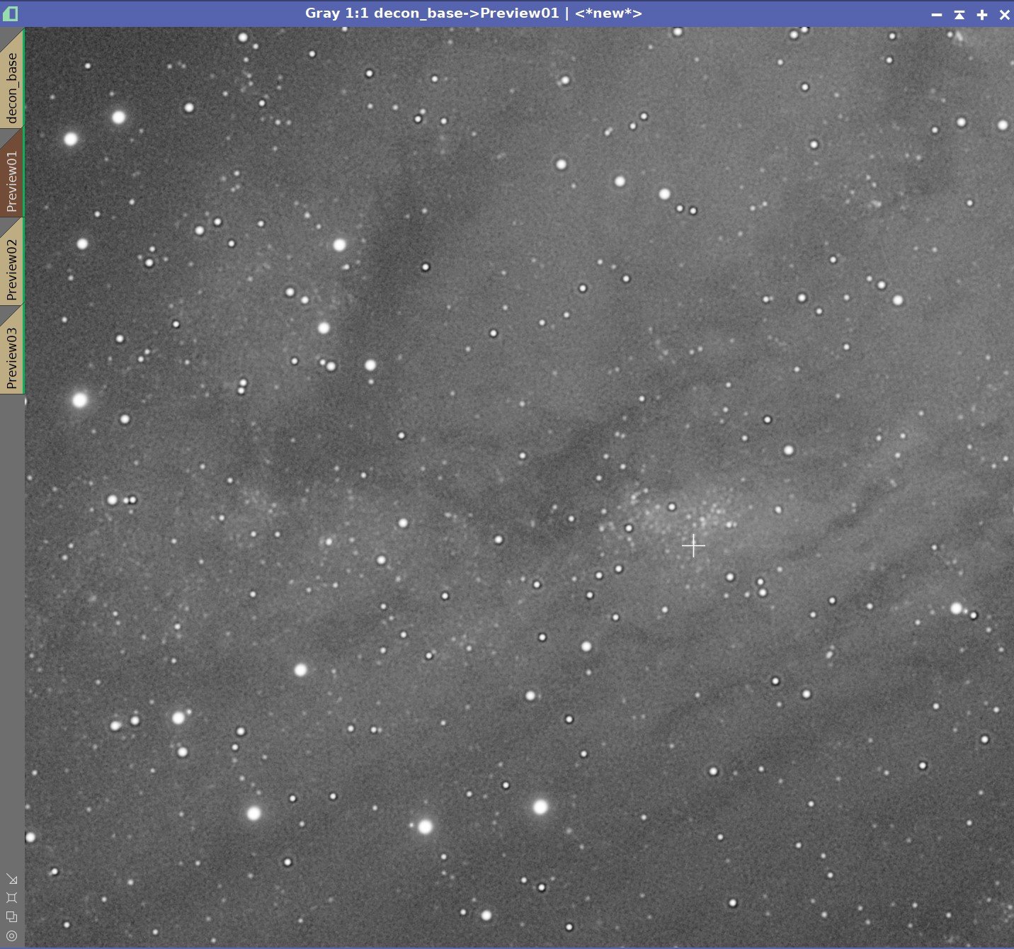
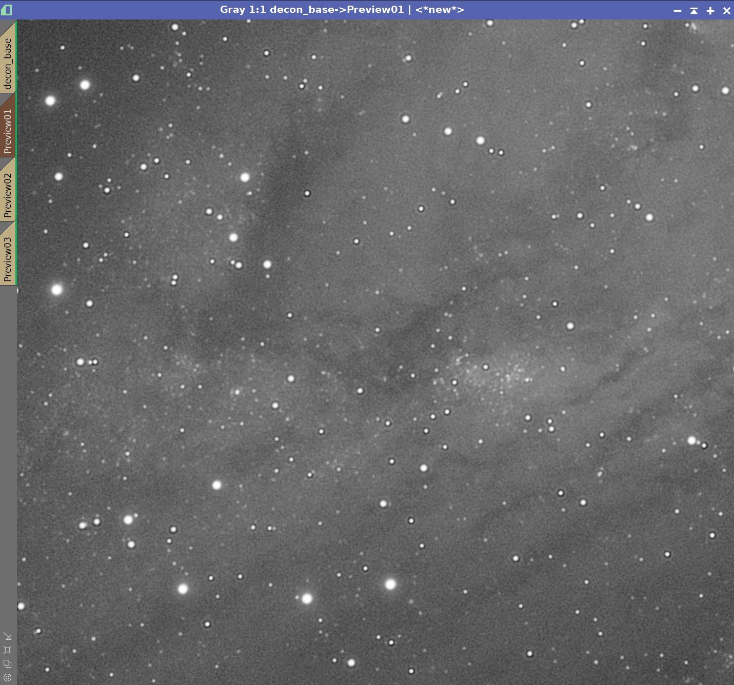
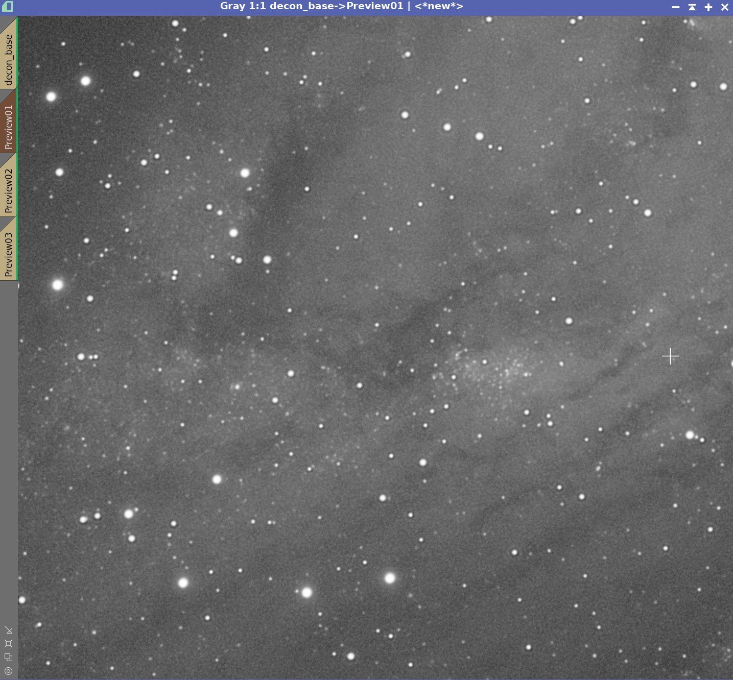
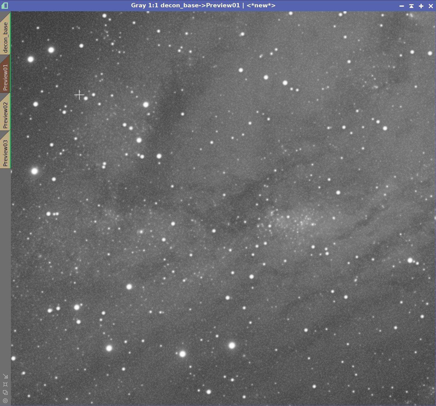
Select Three Preview Regions to Test With

Here are the three previews I selected to work with. And there is that damn cursor again! I have to remember to remove that from the field when I do a screen grab!
Apply the Object mask to the base image:

Here is the whole image showing the Object Mask applied.

Preview 1 with Object Mask applied.

Preview 2 with Object Mask applied.

Preview 3 with Object Mask applied.
Setup the Deconvolution Panel
We followed the same step as with the first example.

Experiment with settings of Global Dark
This time we will do a Global Dark Series with the Local Deringing and Object Mask in place - which is how I normally do it.

Global Dark Series:
0.0001 , 0.001, 0.01, 0.1, 1.0 - with Object Mask and Local Deringing Enabled.
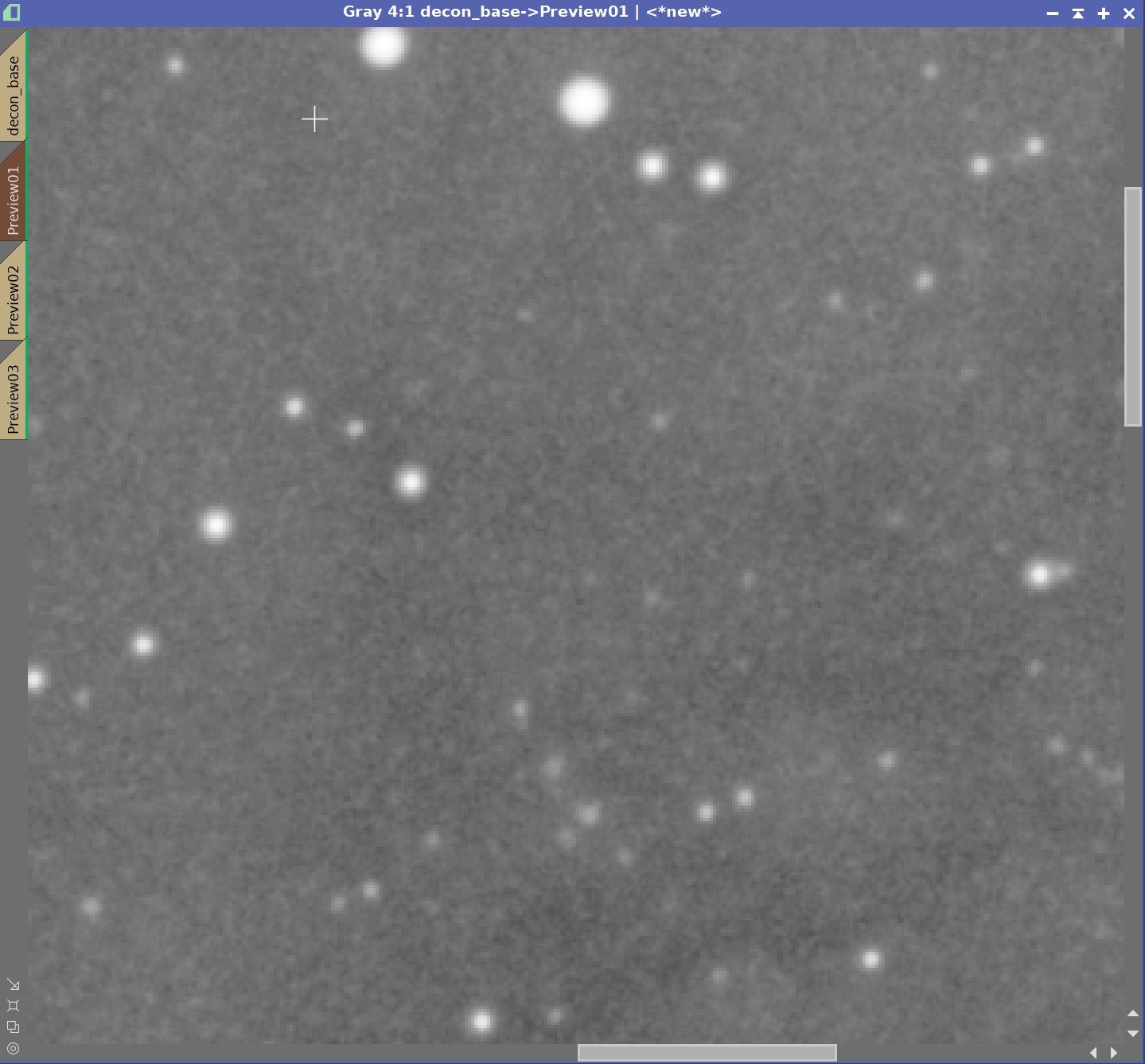
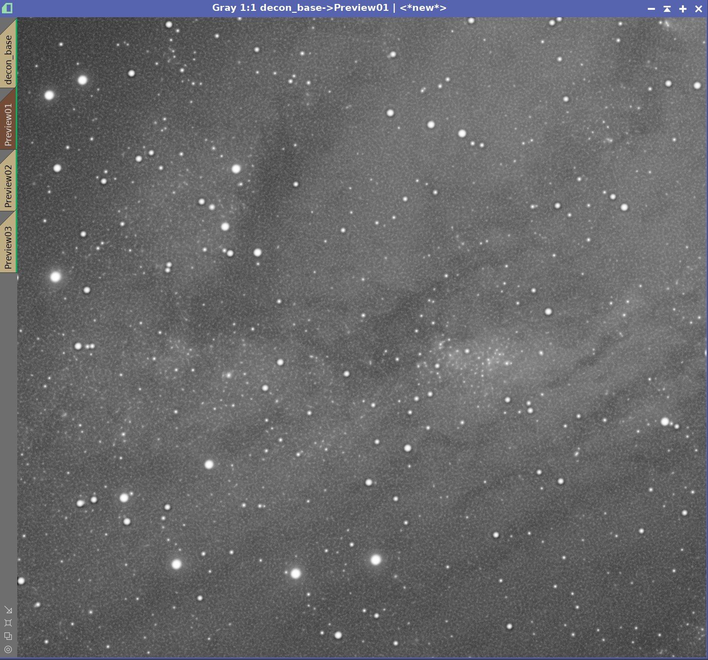
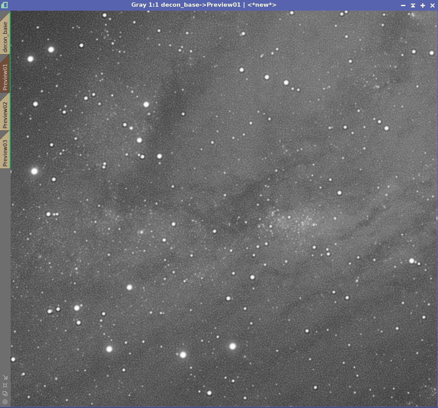
This shows what changes in Global Dark look like for a given preview. At this image resolution, some of the small details are still hard to see. So let’s do that again with a greater level of zoom.
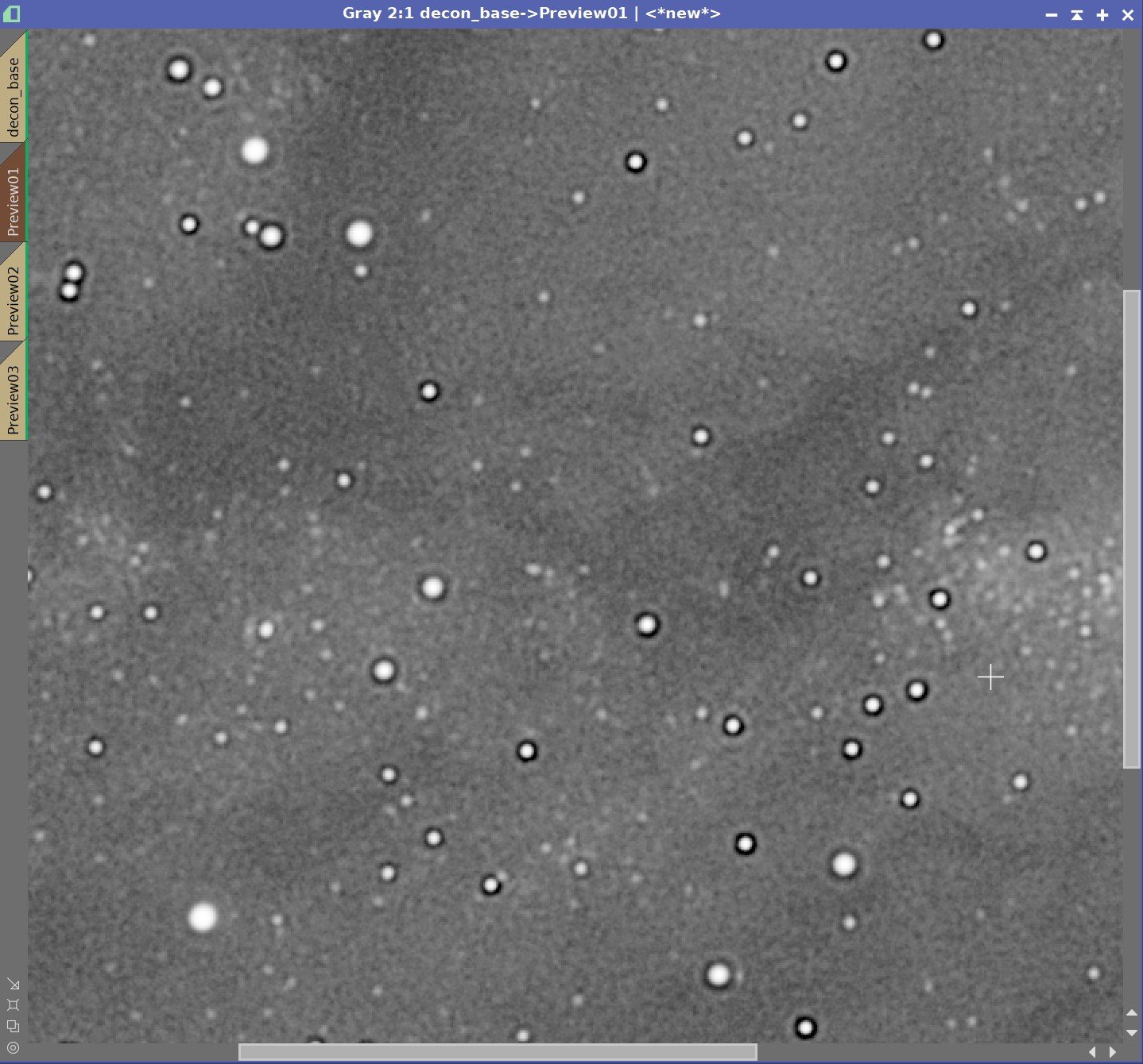


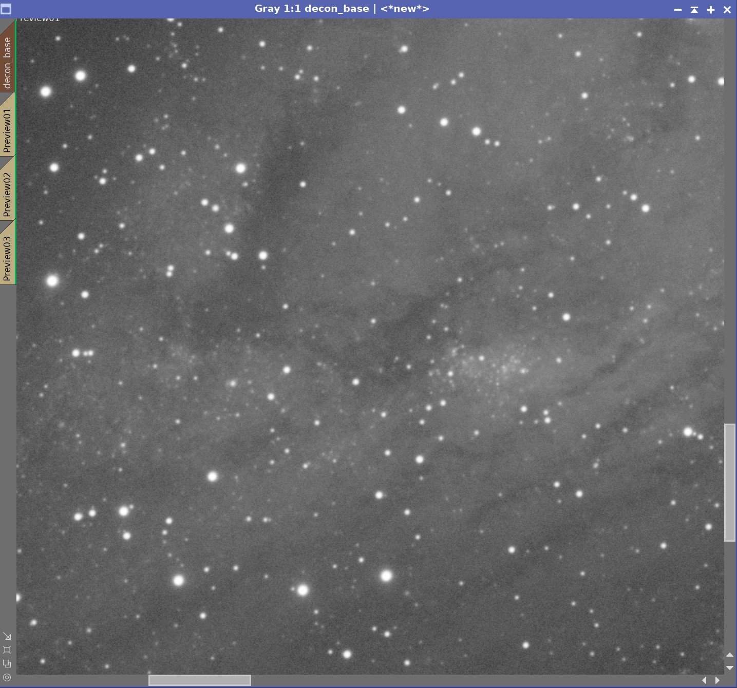
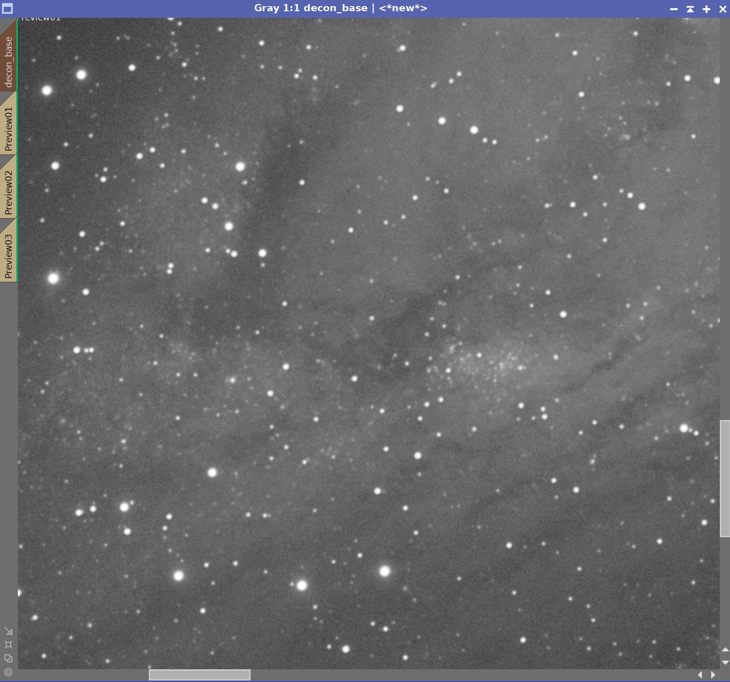
Global Dark Series - This Time Zoomed In More
0.0001, 0.001, 0.01, 0.1, 1.0, - with Object Mask and Local Deringing Enabled.
In this case, the numbers are producing very different results than we saw with our previous example with the Draco Triplet. Dark Rings are forming with much larger values of Global Dark. A value of 0.1 does not look too bad - however a value of 0.01 is starting to show dark rings. The right value is between these two. A final value of 0.07 looked pretty good. This is an order of magnitude larger than what I typically use and I have to believe that the drizzle processing it at play.
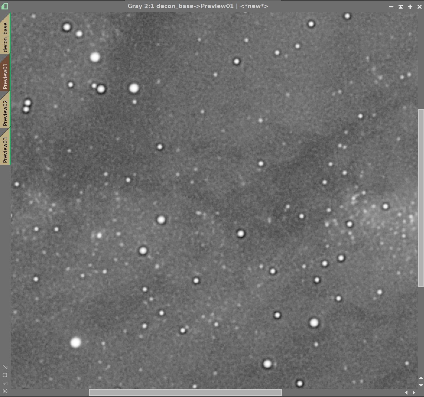
Global Bright
I noticed that I was seeing a sort of stippled background pattern developing the image at my preferred GLobal Dark value. I believe this is a mild case of worms, so I decided to explore the use of the Global Bright Parameter. Now that we have narrowed down the value for Global Dark, we can experiment with iterations.
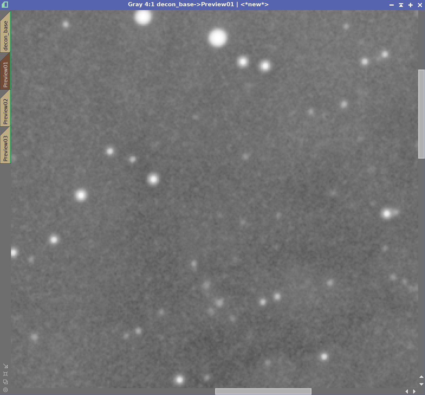
Global Bright Series
Values of 0.0000, 0.0001, 0.0010, 0.0100, 0.1000, 1.0000
With this series, it would appear that we are hiding the pattern with values between 0.1 and 0.01. With further testing I choose the value of 0.05 as the best position.
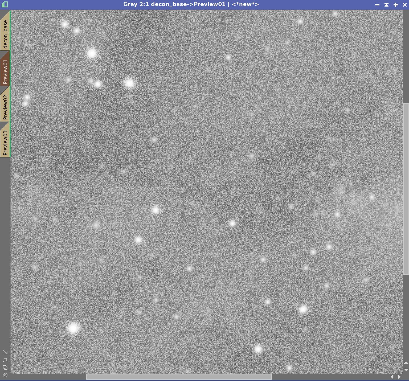
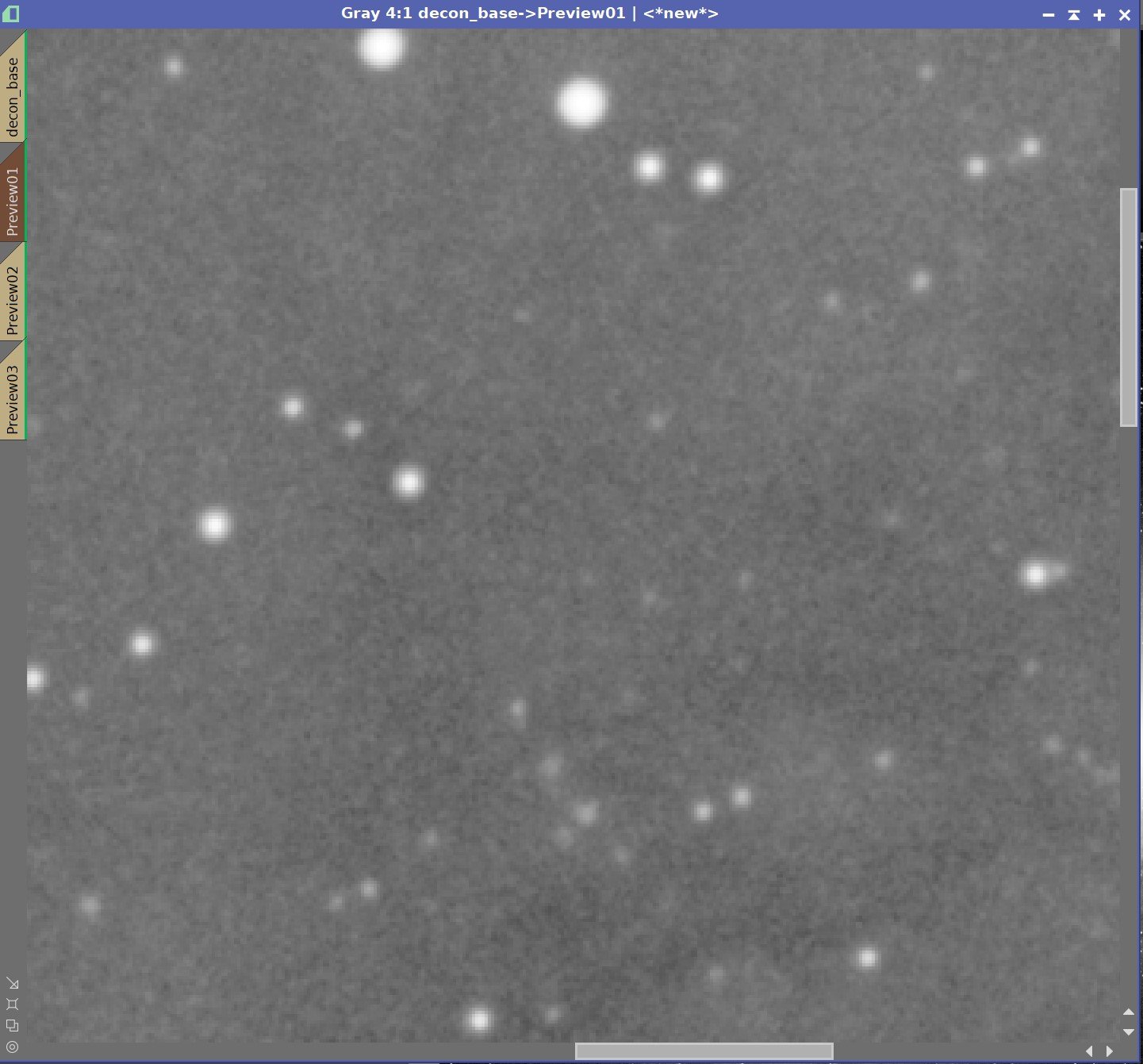
Iterations
The last parameter to test is iterations.

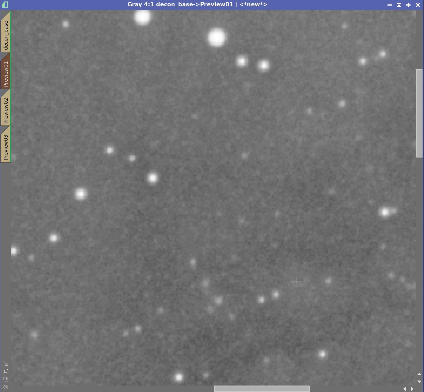
Iteration Series: 20, 40, 60, 80, 100, & 120 Iterations
You may have to zoom in close to see what is going on in this series, but to my eyes, as I increase the number of iterations I see dark rings forming on some stars and areas of lower signal, even though they are protected by the Object mask, are starting to pick up a granular texture that I do not like. For this image, I think I would use 30 to 40 iterations.
At this point, we have selected our value for Global Dark and Global Bright, and we have selected the number of iterations we will run. We can now run Deconvolution on the entire image. Once we have done that, we can carefully check our results and if we are happy, we can move on.
Here is the final setting is for Deconvolution.

Below is the final result we achieved.
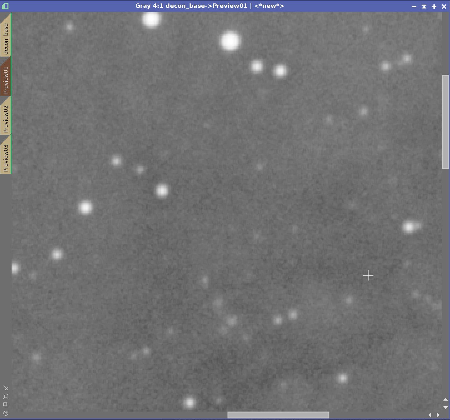
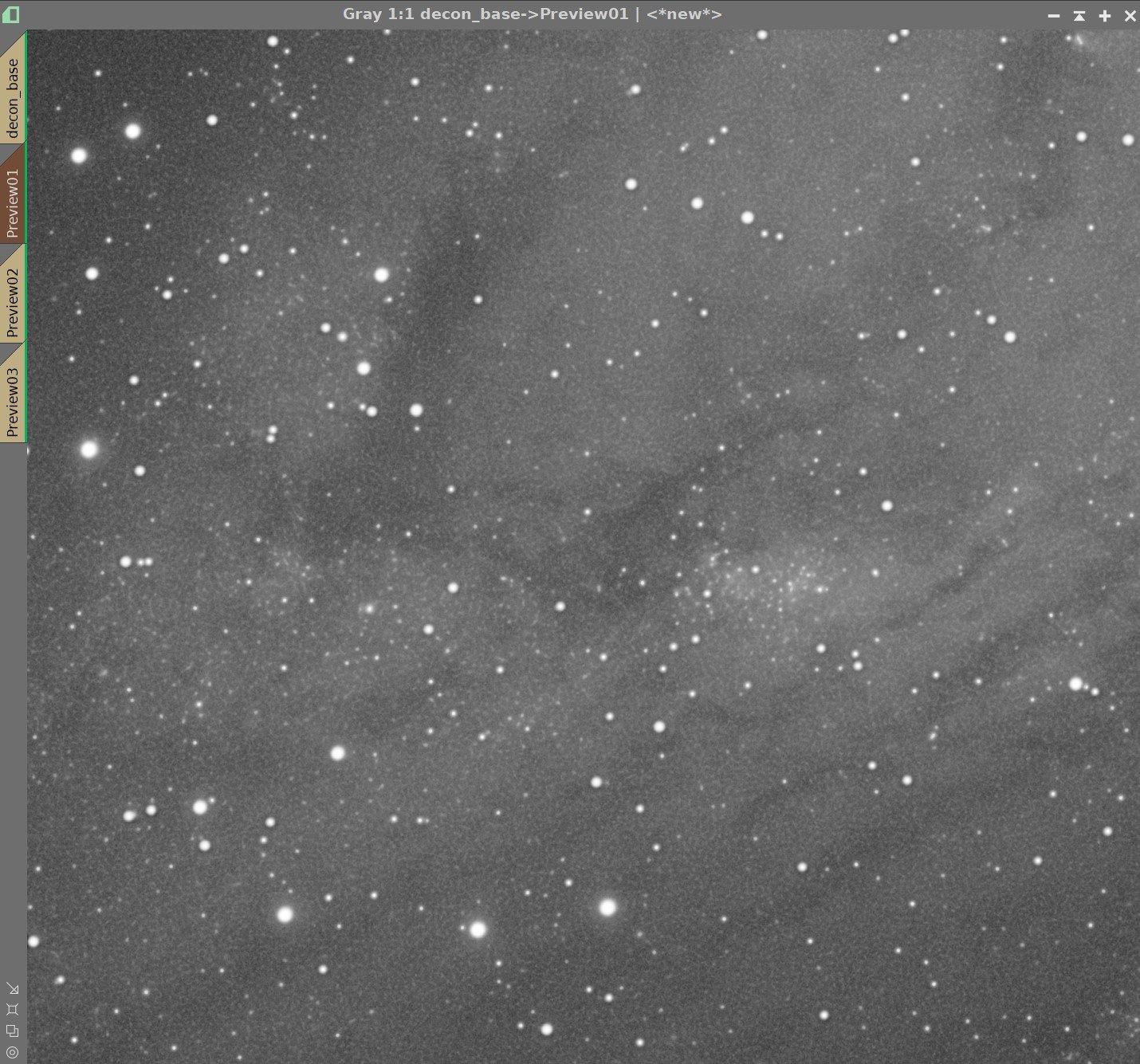
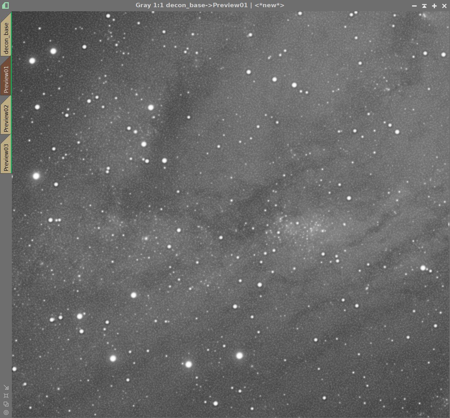
A Final Comparison
Before Deconvolution, After Deconvolution
This was an interesting experiment. There is a definite improvement in this image. It is, however, very subtle! Nothing to write home about!
Even so, we were able to take a pretty sharp image and improve on its sharpness without creating any problematic artifacts.
So can you get some benefit from running Deconvolution on a shorter focal length and a drizzle processed system? Yes, you can - but the value is limited.
The other downside is that the drizzle-processed image is HUGE - and all operations in Pixinsight will be slowed while your CPU cores chew through all of this data. Despite that - I will continue to apply Drizzle processing and Deconvolution to all of my widefield images!
Let’s head back to Part 1 and our Conclusions and Wrapup!
This posting is part of seven-part series: "Using Deconvolution in Pixinsight."
Navigate to other parts of this Series: