
Using Deconvolution in Pixinsight - Part 2: An Overview of PFS and Deconvolution
March 26, 2022

This posting is part of seven-part series: "Using Deconvolution in Pixinsight."
Navigate to other parts of this Series:
Table of Contents Show (Click on lines to navigate)
What is a Point Spread Function?
You probably expected me to jump into talking about what Deconvolution was and how it was implemented in Pixinsight. But I am not going to start there. Rather, I am going to start by talking about Airy Disks and Point Spread Functions (PSFs).
Why? Because If you understand this part - I guarantee that you will understand deconvolution better. Not only that, you will understand WHY you are doing some of the things you have to do in order to get the results that deconvolution can offer.
Stars are so far away (compared with planets from our solar system) that they appear as true point sources.
If we had perfect optics and no atmosphere to look through, we could capture an image with a digital camera and see stars that consisted of a single bright pixel with an abrupt transition to surrounding pixels of the background sky.
(This is obviously a gross simplification as the sensor might be splitting the light from the star across one or more pixels. But you get my drift - as you look at the pixels in the local area of the star, there would be a step-function shift from background intensity to star intensity.)
But in fact, this is not what we see.
As we integrate exposures for a starfield, we see that stars seem to have a “size”. Bright stars seem very big, spanning over a larger area of our sensor, and fainter stars seem to have a smaller footprint. Also, we see that there is a much more gradual transition between the background sky intensity and the star.
This happens, of course, because we do not live in a perfect world.
The energy from the point source has been spread around to a larger area. This “blurring” is due to the effects of the atmosphere and seeing conditions, and the optical effects of our imaging system caused by diffraction, aberrations, fall-off, sensor micro-lensing effects, and so on. Even guiding, dithering, and stacking play into this.
These act together to convolve the image signal and blur it. This blurring changes the image of stars from a point source to an Airy Disk, where light is brightest at the center but falls off as you move away from the center with ever fainter concentric rings forming a skirt around its core. If you were to create a 3D plot of this (X vs. Y vs. intensity), the result would be a Point Spread Function or PSF.
When talking about PSF, one point made in “Mastering Pixinsight” by Rogelio Bernal Andreo, is that a “PSF is not the shape of a star or the image of a star, but a function that describes how the star is shaped.”

A square post function. In a world with perfect optics, a star image would be a true point source and create response from a single pixel where sensor was hit by light from the star. (Image from Wikipedia article on PSFs)

The Airy disk is the typical distribution of light from a point source as image through an optical system with round aperture. The diffraction disks redistributes the light in rings about the center. (Image from Wikipedia article on Airy Disks)

Here is a sample section is taken from one of my own images. Note the varying size of the star images and the apparent Airy Disks that can be seen.

This image was created with the 3DPlot script in Pixinsight of the image to the left. Note the difference in star sizes. Note that some of the biggest ones are chopped off at the top - causing a plateau rather than a peak. This will become an important difference as we talk about estimating PSF models for an image.
The PSF is a map of how the light from the point source was blurred and spread out to form a shape that looks like a curved distribution. You might think that the resulting PSF looks like a normal distribution, but in fact, most stars form a distribution that is more peaked and narrow than a typical Gaussian distribution.
When we talk about star images fitting a distribution type, there are three distributions that are often discussed:
Gaussian Functions defines stars are large and fat and often fit saturated and oversampled stars.
Lorentzian Function defines stars that are very sharp and peaked but have a large fat base.
Moffat Functions sort of fall between the first two functions - not as fat and flat as gaussian stars but also not as peaked as Lorentzian functions and without their large base.
Moffet functions are often the best descriptors for well-formed stars. You will see them listed as different flavors of the Moffat function with a number associated with names (i.e. Moffat7, Moffat 5), these refer to the size of the star. Large numbers look fatter and closer to a gaussian function, while lower numbers look skinnier and closer to the Lorentzian function.


These plots illustrate what various distributions look like - both as a star image, and as a 2D or 3D plot. (Charts created by Jon Rista, used with permission).
While the blurring effect happens for all imaging systems, Astrophotographic systems are somewhat unique in that they regularly contain collections of point sources - Stars!
We can not only see the effect - we can measure it!
Imagine looking at all of the stars contained in a particular image. If you could somehow average the PSF from all of those stars, you could characterize the net effect of the optical and atmospheric forces that shaped that image.
What if you could use this PSF model to reverse the process? A great big “undo” function for your image! What if you could take the energy that has been spread out over a larger area (convolved) and do an inverse function to pull that spread back in?
We would then be able to “de-convolve” the image.
In a discussion with the Twitter #Astrophotogaphy Community on this topic, Tom Boyd made this comment, which I thought was right on the mark:
In this sense, stars are truly magical. They produce beautiful impulse responses (PSFs) from which we can characterize our entire optical system, from source to camera.
— Tom Boyd 🚴♂️ 🇺🇦 🇺🇦 🇺🇦 (@iProvostTom) March 19, 2022
I find it incredibly elegant that our Astro images provide the information to make our images even better!
This type of processing is clearly not a traditional sharpening operation. Sharpening tends to amplify the contrast changes across features and edges.
On the contrary, this kind of operation is more of restoration - a correction for specific distortions made by the system that reveals lost detail.
Deconvolution is designed as an iterative algorithm that uses a modeled PSF to do just that.
Before we get further into deconvolution, let’s explore PSFs a bit more.
Creating an Estimate of PSF
I should stress at this point that a PSF model is not a precise thing. It is simply the best estimate that we can make for a given image.
So if the PSF for an individual star is its own characterization of the optical distortions for a given system - then taking the PSFs for all of the stars in an image would be an even better way to estimate the average response - right?
Well… no.
Often is it better to use a smaller sampling of stars to form a PSF estimate. Why is this true?
It may be computationally inconvenient to crunch down on all of the stars contained in an image. We really don’t need that many.
Not all stars are equally well-formed and we really want to eliminate those stars that have distortions that make them poor candidates for computing the final PSF.
So, what kind of stars would we want to avoid?
Saturated Stars
It’s easy to overexpose stars, especially when we’re dealing with bright stars. A saturated star looks like its peak has been chopped off - leaving behind a broad flat plateau. Once you saturate the sensor, it no longer has the ability to respond to higher signal levels so the natural PSF is truncated by this loss of response. Such stars are distorted and are no longer representative of the system optical response.
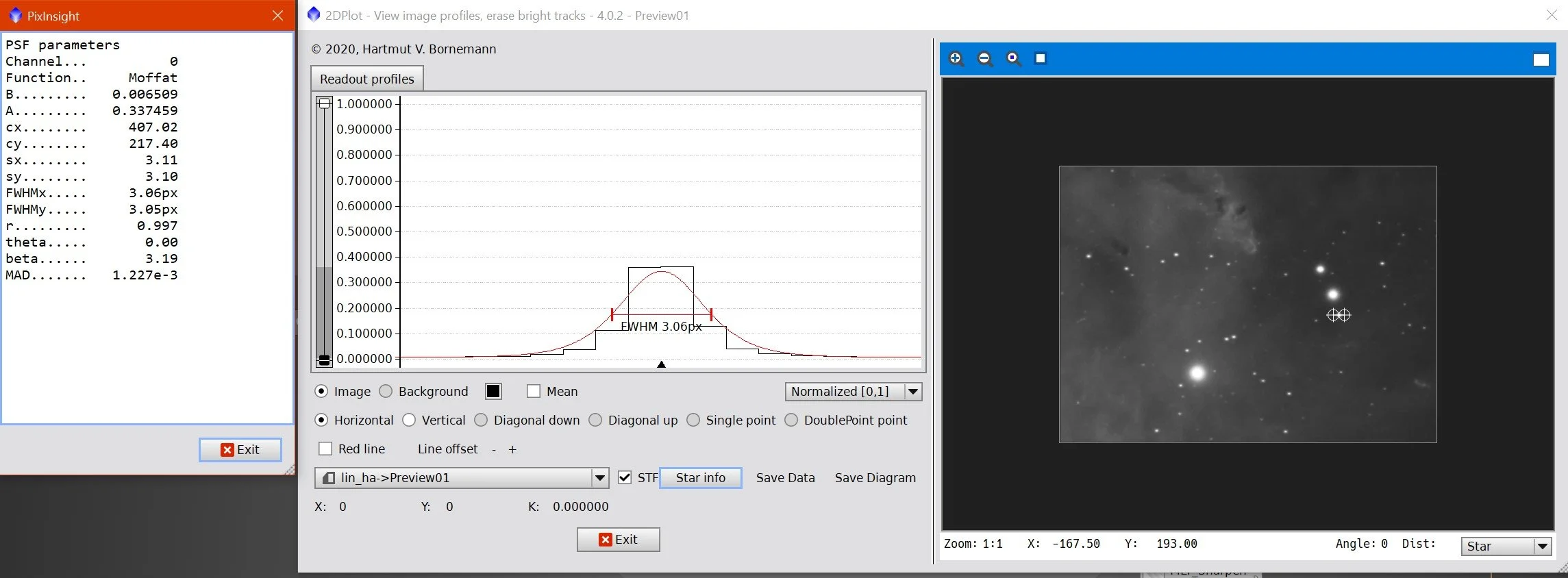
This is the 2DPlot script by Hartmut Bornemann in Pixinsight. Here we are looking at a well-behaved star image (the selected star can be seen indicted in the image to right). The peak intensity is only halfway up the scale and nothing is distorted. This would be a great star to use for estimating PSF.

This 2DPlot (Script by Hartmut Bornemann)is from a pretty bright star. As you can see, the star has saturated the sensor, and the plot is chopped off at the top and presents a distorted PSF. This would not be a good star to use for PSF Estimations.
By the same token, saturated stars don’t do well if you run Deconvolution on them. Their distortions will drive ringing and artifacts to form. So Saturated stars are bad actors when estimating a PSF model and when trying to enhance the image.
Faint Under-Exposed Stars
This is just the opposite of the saturated star case. Here we have a very faint star that is just barely registering and forming an image. Would it make sense to use the PSF of such star images when building a PSF model for the whole image?
Probably not. Since the star is just barely registering, it is likely to not show enough detail in its PSF to be a useful measure of the system performance. The contribution of noise would further complicate this issue. Here, the clipping is occurring at the other end of the scale. The difference between a very faint star and just a noise blip is pretty small. Neither will help you to form a good PSF model. Nor is it something that you would want deconvolution to operate on.

Here is a very faint star. There is just not enough detail in the star’s PDF to be useful.
Aberrations
Sometimes the response of the system is not consistent across the entire frame or across the color spectrum.
Spherical Aberrations can cause distortions at the edge of the field. Clearly, including stars that have such optical distortions into the estimate for the PSF is not the best thing to do. My advice here is limited - but it would be best to use a field flattener on your scope to correct for these issues before you even try to collect data. Short of this, I would try to avoid stars from the edge of the field when you are estimating your PSF.
Chromatic Aberrations are pretty much nonexistent for reflecting telescopes and can be very well controlled for three and some two-element lens refractor systems. However, if you are dealing with Chromatic Aberration, you have a situation where the best estimate of the PSF for an image might well be different for the Red, Green, and Blue Images. In this case, it may well be worthwhile to treat each color layer separately. This would allow you to create a unique Red, Green, and Blue PSF that when used by Deconvolution, may improve things. I have not had to deal with this issue myself, but if I did, I would certainly be interested in giving this a try.
Encumbered Stars
It is best to deal with stars that are well-formed and isolated. Stars that are buried in bright nebulae, or the arms of a galaxy, or even close double star pair - are not as clean to work with and it is best to avoid them.
Small Galaxies
Some star fields are scattered with faint tiny galaxies that might be mistaken for stars. Since these are not true point sources, you should avoid them.
Other image Considerations for PSF Estimation and Deconvolution
There are other factors that come into play as we consider Estimating and using PSFs and Convolutions.
Signal-To-Noise
It should not surprise you to learn that images with a better signal-to-noise ratio will do better than images with a lower one when it comes to deconvolution. This also plays out within an image as well. Regions or specific objects within the image will do better if they have a higher signal level, Whereas areas that are more noise dominant will react to that noise - often growing clumps of noise that do nothing to enhance the image.
Camera Sampling
PSF models and Deconvolution do best when there is plenty of pixel data to describe the Airy disc of each star.
When you are choosing a camera that will work well with your telescope, you look for a combination of camera-telescope that will provide the right sampling level for your images.
A great tool for determining your sampling level is this calculator: http://astronomy.tools/calculators/ccd_suitability
If you are undersampling your images, small faint stars may be seen as a single square pixel. Brighter stars can have a “boxy” appearance with few pixels describing their PSF. Undersampled images are starved for information content. It should not be a surprise that images that are undersampled may not do well with deconvolution. The PSF model you can compute with be coarse and blocky. When you try to apply deconvolution, your results will have issues. Deconvolution on undersampled images will increase the contrast on key signal features but ultimately it will make the image look even more blocky - emphasizing the undersampled nature of the image.

This chart showing examples of sampling is from the ZWO Website.
Images that are well sampled or even oversampled allow you to build an effective PSF model and will also allow you to achieve better results when deconvolution is run. Be aware of this and make sure your system has adequate sampling.
If your system is sightly undersampled, then one option you have is to Drizzle process your image during the pre-processing phase. This can increase the effective resolution and thus improve your effective sampling rate for an image.
The original paper on Drizzle Processing (with thanks to Paul Leyland!)
Linear vs Non-Linear Images
When the sensor first captures your image, you are still in the linear response domain. The sensor has captured data as it was seen and all relationships are preserved. Once you take the image nonlinear, the relationships of various attributes become distorted and the original patterns are lost. Therefore, estimates the system PSF and applying deconvolution should be confined to when the image is in a linear state.
Non-Star Areas
What I am talking about here are image areas that are not stars. These could be areas of nebulosity or even background sky. Since these are not point sources, they offer no real value when trying to estimate the PSF for the image.
However, they can be operated on by deconvolution using a PSF estimate based on the stars in your image. As previously noted, strong signal areas of the image can indeed be improved by deconvolution, but applying deconvolution to the low signal areas - areas that have great noise - should be avoided. The noise would be acted upon to redistribute energy in a way that would "enhance" it (i.e. make it more noticeable). We will want to avoid that - and the deconvolution tools have ways to manage this.
Focal Length
The conventional wisdom is that the best results from Deconvolution are delivered with systems that have longer focal lengths of bout 1000mm or longer. I think the assumption here is that shorter focal length wide-field systems are likely to have very coarse image scales and be very undersampled.
I tend to try and use Deconvolution for all of my images. I run three telescopes at the same time, and these have focal lengths of 920mm, 1080mm, and 400mm. My own experience tends to confirm this - I tend to get only modest sharpening with the 400mm scope, with better results being seen with the two longer focal length instruments. Recently I started drizzle-processing the images from the 400mm system. We will see if this helps the situation any.
I will be running one example image from each of my telescope systems, so we will see what can be done for each.
So What is Deconvolution?
Deconvolution is a mathematical algorithm that employs an inverse point spread function to redistribute pixel intensities over a grid of pixels attempting to reverse the blurring effects inherent in an optical path.
The foundations for deconvolution were largely laid by Norbert Wiener of the Massachusetts Institute of Technology by his work during World War II. During the war, this work was classified. After the war, he published his book “Extrapolation, Interpolation, and Smoothing of Stationary Time Series” (1949) which documented the methodology for the first time. Deconvolution has wide application for a diverse set of signal processing domains.
Deconvolution Algorithms work iteratively, and with the proper image parameters, the changes made for each iteration will converge.
When applied across an image, the benefits can be tainted or limited because of image artifacts that may be generated due to noise or responding to portions of the image that are not well represented by the PSF model in use. This is because Deconvolution is done in the frequency domain rather than the spatial domain. It can react quite strongly to discontinuities that can found in that domain.
When iterative results begin to diverge rather than converge, some spectacularly bad artifacts can be generated.
Pixinsight has implemented several deconvolution algorithms that can be selected from the Deconvolution Tool Panel. It also has mechanisms and parameters that allow the algorithm to be run in such a way as to avoid issues common to deconvolution.
The algorithms supported are:
Richardson-Lucy: typically used for deepsky images.
Van Citter: typically used for high-resolution lunar and planetary images.
Regularized Richardson-Lucy: Regularized version of the Richardson-Lucy algorithm.
Regularized Van Citter: Regularized version of the Van Citter algorithm.
According to The Officially Unofficial Reference Guide, “Regularized versions of an algorithm work by separating significant image structures from the noise at each deconvolution iteration. Significant structures are kept and the noise is discarded or attenuated.”
The challenge is understanding how to use this powerful tool. There is no documentation available for the process, so you will need to seek out other sources to learn about its use. (Hopefully, this posting will help!)
But first, let's talk about where in the process flow deconvolution should be applied. This will be covered in the next section.
This posting is part of seven-part series: "Using Deconvolution in Pixinsight."
Navigate to other parts of this Series: