SH2-173 - The Phantom of the Opera Nebula | 15.77 hours of SHOrgb
Date: October 7, 2026
Cosgrove’s Cosmos Catalog ➤#0169
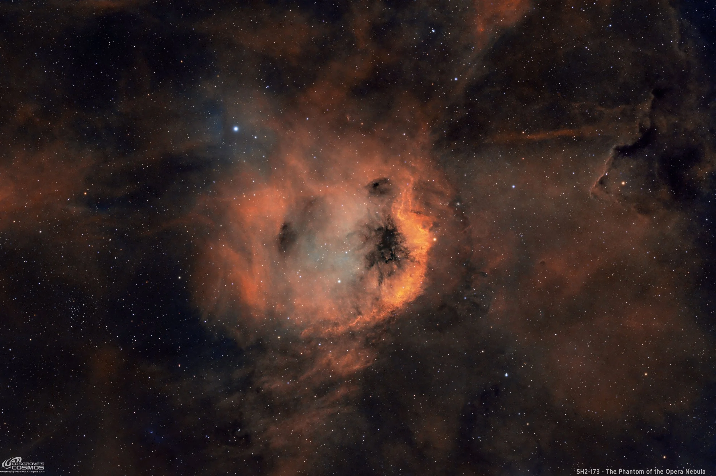
SH2-173 - The Phantom of the Opera Nebula (Click the image for a high-resolution version on AstroBin.com.)
Sh2-173 — the Phantom of the Opera Nebula, where glowing gas and dark dust form a ghostly mask amid the star fields of Cassiopeia.
🔭 Project Summary
Target: Sh2-173 — The Phantom of the Opera Nebula / Sharpless 173 / Simeis 21 / LBN 593
Principal Ionizing Star: BD+60 39 (ALS 6151), an O9V star
Capture Dates: September 6, 11, and 14, 2026
Constellation: Cassiopeia • Distance: ≈ 8,200 light-years (± 1,600 light-years)
Type: H II emission nebula associated with molecular clouds and young stars in the Milky Way’s Perseus spiral arm
Imaging Period: September 6–14, 2026 • Total Integration: 15 h 46 m 00 s (SHO narrowband + RGB)
Filters: Ha · OIII · SII (Astronomik 36 mm 6 nm) + R · G · B (ZWO 36 mm LRGB Gen II)
Telescope: Astro-Physics 155 mm Starfire EDFS f/5.3
Camera: ZWO ASI2600MM-Pro (−15 °C; Gain 100 narrowband, Gain 0 RGB)
Pier / Support: A Custom steel pier
Processing: PixInsight (SHO narrowband + RGB) & Photoshop
Location: Whispering Skies Observatory · Honeoye Falls, NY (USA)
Acquisition notes: Ha: 70 × 300 s; OIII: 39 × 300 s; SII: 69 × 300 s at Gain 100. R: 16 × 90 s; G: 16 × 90 s; B: 16 × 30 s at Gain 0. All exposures bin 1×1 at −15 °C; 226 light frames totaling 15 h 46 m 00 s after culling bad or questionable subs.
Image note: This SHO narrowband and RGB image captures Sh2-173, the Phantom of the Opera Nebula, with a bright orange-gold rim, a softly glowing interior, and intricate dark markings that suggest a ghostly mask. Faint surrounding emission and dark lanes extend across the Cassiopeia star field, placing the central nebula within a broader landscape of interstellar gas and dust.
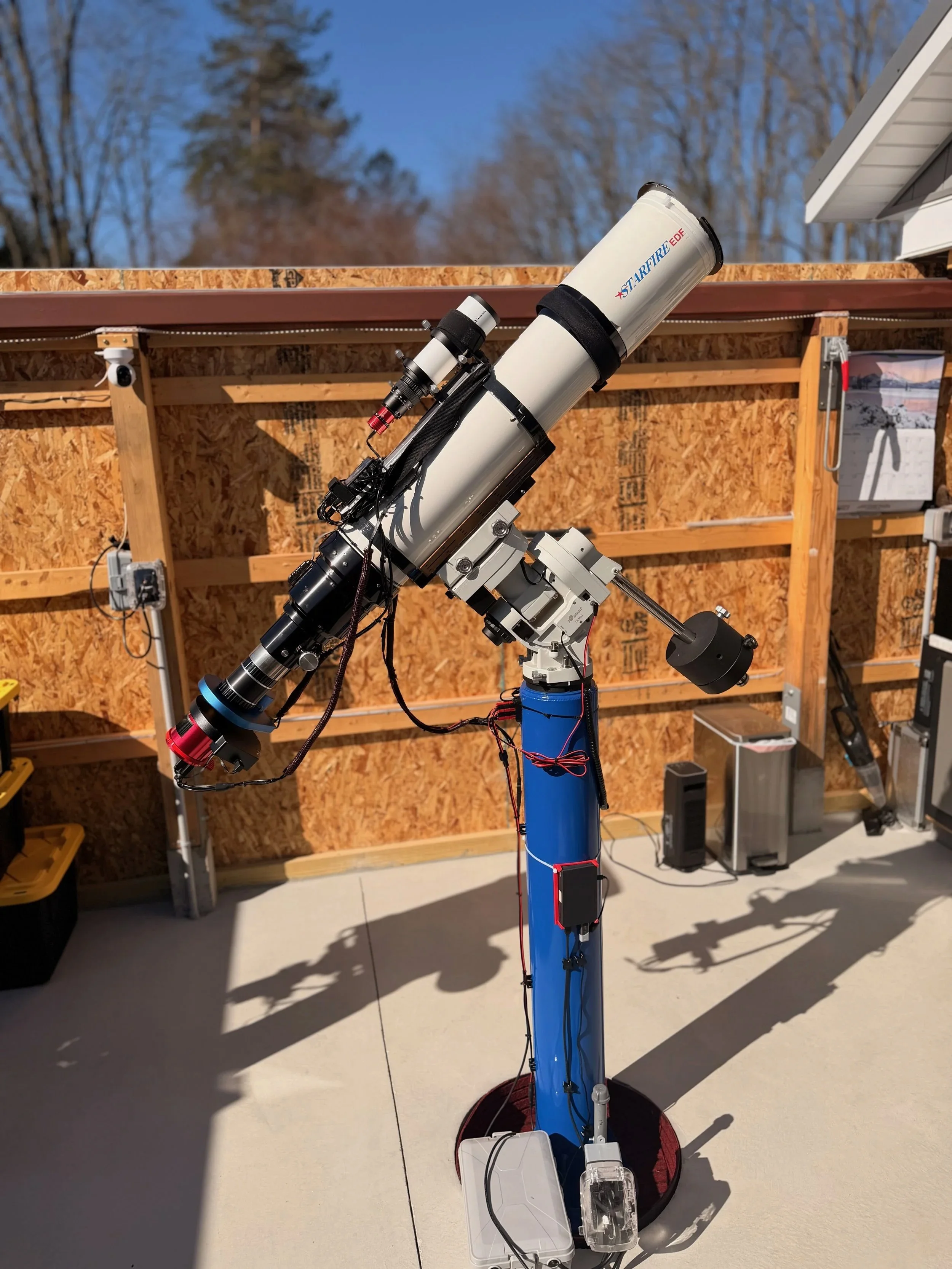
The AP155 platform used for this project.. (click on image to go to the blog entry for this scope)
📸 Capture Details
Nights: September 6, 11, and 14, 2026
| Channel / Filter | Frames × Exposure | Settings | Total |
|---|---|---|---|
| Ha — Astronomik 6 nm Hydrogen-alpha (36 mm unmounted) | 70 × 300 s | bin 1×1 • −15 °C • Gain 100 | 5 h 50 m |
| OIII — Astronomik 6 nm Oxygen III (36 mm unmounted) | 39 × 300 s | bin 1×1 • −15 °C • Gain 100 | 3 h 15 m |
| SII — Astronomik 6 nm Sulfur II (36 mm unmounted) | 69 × 300 s | bin 1×1 • −15 °C • Gain 100 | 5 h 45 m |
| R — ZWO Red Gen II (36 mm unmounted) | 16 × 90 s | bin 1×1 • −15 °C • Gain 0 | 24 m |
| G — ZWO Green Gen II (36 mm unmounted) | 16 × 90 s | bin 1×1 • −15 °C • Gain 0 | 24 m |
| B — ZWO Blue Gen II (36 mm unmounted) | 16 × 30 s | bin 1×1 • −15 °C • Gain 0 | 8 m |
| Total Integration (after culling): 15 h 46 m 00 s (SHO narrowband + RGB) | |||
Frame counts reflect the 226 light frames retained after bad or questionable subs were culled.
Calibration Frames
- 25 × dark frames @ 300 s, bin 1×1, −15 °C, Gain 100
- 25 × dark frames @ 90 s, bin 1×1, −15 °C, Gain 0
- 25 × dark frames @ 30 s, bin 1×1, −15 °C, Gain 0
- 30 × dark-flats @ each flat exposure time, bin 1×1, −15 °C; Gain 0 for RGB and Gain 100 for narrowband
- Flats: 15 each — Ha, OIII, SII, R, G, B
Table of Contents Show (Click on lines to navigate)
Annotated Image
This annotated image began with PixInsight’s ImageSolver and FinderChart tools, then was enhanced to show additional features.
The Location in the Sky
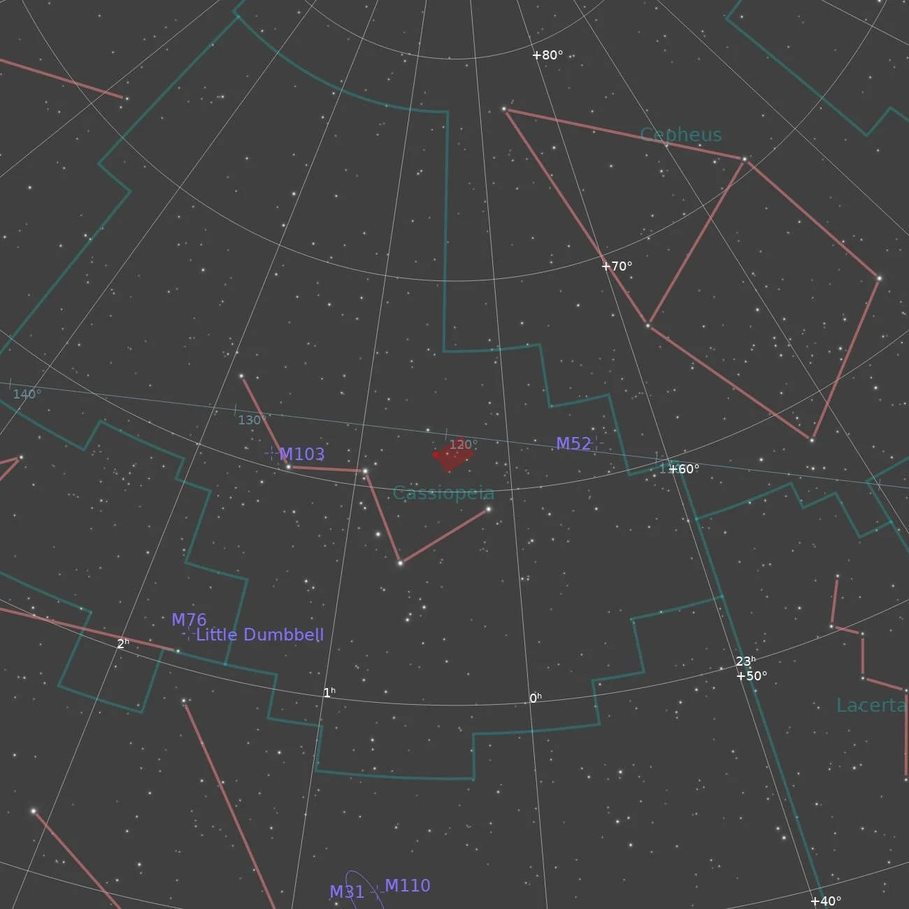
This finder chart shows the location of SH2-173 in Cassiopeia. It was created with the ImageSolver and FinderChart scripts in PixInsight.
🎭 Introduction
Some nebulae require a little imagination to see the shape behind their nickname. Sh2-173 gives us a pretty good starting point. A curved rim of glowing gas, a pale interior, and dark markings cutting across its face create the appearance of a ghostly mask suspended against the stars.
This project combines 15.75 hours of SHO narrowband and RGB data, captured with my Astro-Physics 155mm refractor, to reveal the Phantom of the Opera Nebula and the faint nebulosity surrounding it.
About the Target
🌌 Overview — What and Where Is Sh2-173?
Sh2-173, commonly called the Phantom of the Opera Nebula, is a faint emission nebula in Cassiopeia. It lies approximately three degrees north of Caph, the star marking the western end of Cassiopeia’s familiar “W,” in the direction of the Milky Way’s Perseus spiral arm. Location and identification
It is classified as an H II region: a cloud of interstellar gas in which energetic radiation from hot stars has ionized the hydrogen. The “H” denotes hydrogen, and “II” indicates its ionized state. Its designation places it among the emission regions recorded in Stewart Sharpless’s second catalog. Sharpless’s catalog of H II regions
The recognizable Phantom occupies the central part of this image, but the surrounding field adds considerably to its appearance. A bright curved rim wraps around a softer interior, dark markings interrupt the glow, and faint reddish structures extend outward across the frame. Together, these features suggest a mask emerging from a much larger cloud.
📜 History — From Photographic Plates to the Phantom
The discovery of this faint nebula is generally credited to Grigory Shajn and Vera Gaze, working at the Simeis Observatory in Crimea during the early 1950s. Their photographic surveys revealed numerous clouds of glowing interstellar gas, including the object known as Simeis 21. The available historical accounts place its discovery within that survey work rather than on a precisely documented observing night. Historical overview
American astronomer Stewart Sharpless later included the nebula in his 1953 catalog as entry 121, with a reference to the earlier Simeis designation. Sharpless examined photographic plates taken with Palomar’s 48-inch Schmidt telescope, identifying emission nebulae and recording their appearance and associated hot stars. This systematic photographic survey allowed faint, extended structures to be studied across large areas of the Milky Way. Sharpless’s original 1953 catalog
In 1959, Sharpless published his expanded A Catalogue of H II Regions, giving the nebula the designation we use today: Sh2-173. “Sh2” identifies the second Sharpless catalog, and “173” is its entry number. That date marks its inclusion in the revised catalog, rather than its original discovery. Sharpless’s 1959 catalog
The name Phantom of the Opera Nebula came later as an informal description of its appearance. Its bright, curved outline and dark markings suggest the masked face associated with The Phantom of the Opera. The nickname appears in astrophotography presentations, including Anthony Ayiomamitis’s page featuring his 2011 image, but I have not found a reliable attribution for who introduced it or when. Ayiomamitis’s image and description
🔬 Science — What We Know, and How We Know It
Measuring its distance
Astronomers estimate distances to regions like Sh2-173 by studying their associated stars. Spectra establish stellar classifications, while brightness and color measurements help account for intervening dust. Comparing the stars’ expected intrinsic brightness with their observed brightness then provides a distance estimate. Russeil and colleagues used this approach in their study of northern H II regions. They also investigated departures from ordinary Galactic rotation, which complicate distances inferred from gas velocities alone. Russeil, Adami & Georgelin, 2007
A subsequent study adopted 2.5 ± 0.5 kiloparsecs, approximately 8,200 ± 1,600 light-years. At that distance, its measured ionized region spans roughly 60 light-years. Cichowolski et al., 2009
Identifying the star that powers it
Radio measurements confirm emission from ionized gas and allow astronomers to estimate the ultraviolet radiation needed to sustain it. Comparing that requirement with stellar models shows that BD+60 39, an O9V star, can supply enough ionizing photons by itself. Ionization analysis
Mapping the material around the glow
Observations of neutral hydrogen at 21 centimeters, carbon monoxide emission, and infrared dust emission reveal surrounding material invisible in an ordinary photograph. Matching structures and gas velocities connect the nebula with adjacent atomic and molecular gas; infrared maps reveal a boundary affected by stellar ultraviolet radiation. Multiwavelength observations
Searching for stars still forming
Infrared colors and positions relative to molecular clouds identified 46 candidate young stellar objects probably associated with Sh2-173. These are survey-selected candidates, rather than 46 individually confirmed newborn stars. Young-star search
Reconstructing its evolution
Expansion models suggest an age of 600,000–1,000,000 years. Its position beside a larger, older gas shell supports a possible sequence of triggered star formation. The ages and spatial arrangement support this interpretation, but do not prove that one generation caused the next. Evolutionary analysis
✨ What Stands Out in This Image
The brightest orange and gold emission curls around the right side of the central structure, while softer tones fill the interior. An intricate dark feature cuts into the bright rim, helping define the Phantom’s face.
Beyond that recognizable shape, faint reddish nebulosity spreads across the frame. The mask catches the eye first, but the surrounding wisps and dark lanes give the image much of its depth.
About the Project
Planning and Weather
I’ve been doing astrophotography for about 7 years, and I would have to say 2026 has been the worst year, weather-wise, by far!
August is typically a very hot, dry month for us, and that can lead to clear, dark nights. However, these nights have relatively few hours of true darkness. Then September comes along and the nights get longer, and we often have some really nice stable periods. These long, clear nights are outstanding for capturing data.
But this year, August was very stormy, unsettled, and cloudy! We also had smoke from forest fires drifting our way. September was just as unsettled.
Despite this, I found three nights where I could catch photons. The weather apps predicted marginal conditions for each night, but beggars cannot be choosers, so I fired up the gear each night expecting to be shut down after a few hours. I was fortunate to keep imaging through the night, although intermittent thin clouds, smoke, and heavy dew affected the conditions.
I say clear skies, but in fact we did have some thin clouds coming through, some light smoke, and the heaviest dew I have seen in many years. So things were not ideal!
Target Selection
For this project, I was looking for a target for my AP155 platform.
I often hunt for targets in the Sharpless Catalog, and often find objects that I have never heard of that look very interesting.
As I scanned the constellations well placed for this time of year, I went through Sharpless objects in Cassiopeia and came across Sh2-I73. As I looked at the catalog plate, the nebula looked like the face of a polar bear or maybe a dog. As I researched it further, I found that it was called the Phantom of the Opera Nebula. Not what I was expecting.
All I could see was the face of a puppy dog! With some effort, I suddenly saw the image of a mask looking up into the sky. But it took a focused change of perspective to see this shape! Talk about your inkblot tests!
But this made me curious about the target, and once I am curious about something, I go after it.
It turned out to be well-sized for my AP155 scope, and that cinched it!
I planned to capture a full narrowband image, using limited subs to collect RGB stars.
Data Collection
I opened the roof around 7 pm, which helped cool things down a bit.
The days weren't as warm, and the evenings were getting cooler. I had been using a camera cooler setting of -10 degrees because I knew they couldn't hit -15 with the warm nights we had earlier in the year. But with teh cooler nights, I went back to my standard aim of −15 °C.
My plan was to use 300-second narrowband subs and 30-second RGB subs. I wanted to collect a limited number of RGB subs, so I set the limit to 16 for each filter. Then I would go back to collecting the narrowband subs.
That's when I messed up. I copied an old NINA sequence file from a previous shoot and changed things that needed updating. In the process, I changed some 90-second RGB subs to 30-second subs. I must have gotten distracted because Blue exposures were 30 seconds, while Red and Green exposures were 90 seconds.
Whoops!
Data collection over the three nights went very well, with no other glitches besides my NINA sequence setup. Now that the AP155 has been well balanced and dialed in, tracking has been excellent, as have been my results!
Calibration Frames
A few nights after collecting the last data, I decided to grab a complete set of calibration data.
With the Wanderer Astro cover, I could easily do the entire process remotely. Talk about convenience!
I collected a complete set of darks, dark flats, and flats for this project.
Pre-Processing
As always, I bliked all of the data, including the cal files. A handful of frames were obscured by clouds, but most were fine, so I left them in the collection.
I noted a very strong signal in Ha, a weak signal in SII, and almost no signal in OIII. This made me wonder whether it was a mistake to collect the OIII data. But I have thought this before, only to find that after stacking, something was there. So I had to wait and see.
But an HSS processing approach might be better than my standard SHO approach.
In SHO, SII supplies red, Hα supplies green, and OIII supplies blue. In HSS, Hα supplies red and SII supplies both green and blue. Separately processed RGB data supplies the stars.
I then used WBPP to process my frames and create the master images. The integrated OIII master showed very little detectable nebular signal in this dataset. There were hints there but not much else.
So I had to decide which way to go: HSS or SHO?
In the end, I decided to do both approaches to a point and pick the one that I thought was most visually pleasing.
Post-Processing
Processing for HSS vs SHO is very similar. The stars would be formed from the RGB data, so that part was the same. Both versions shared the same basic linear-processing workflow and RGB-star preparation, but I adjusted their nonlinear color, tone, and contrast separately.
So I used my typical narrowband + RGB star workflow that looks something like this:
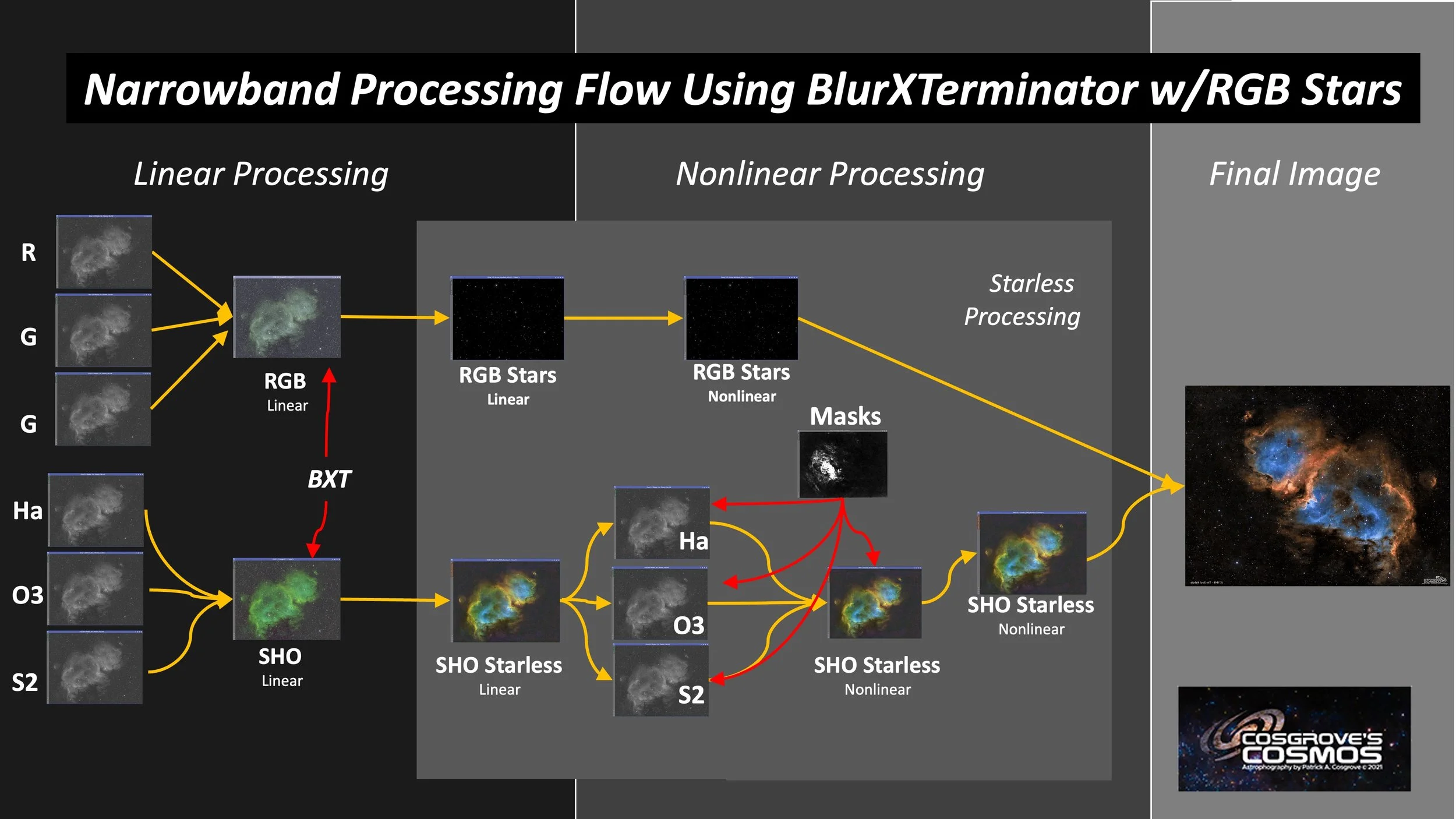
My typical SHO + RGB Starless Workflow.
The other aspect is that I expected to use PixInsight processing scripts I created for this project.
I have already published the Astro Color Mixer and Astro Contrast Enhancer scripts, so anyone can use them. (Information on these can be found on my Software Utilities Page)
But I have also been developing two other utilities that are not ready for release yet. For that, I apologize - my detailed processing walkthrough for this image will show their use, but you can’t use them as of yet. But hopefully that will change in the next few weeks as I complete and release them.
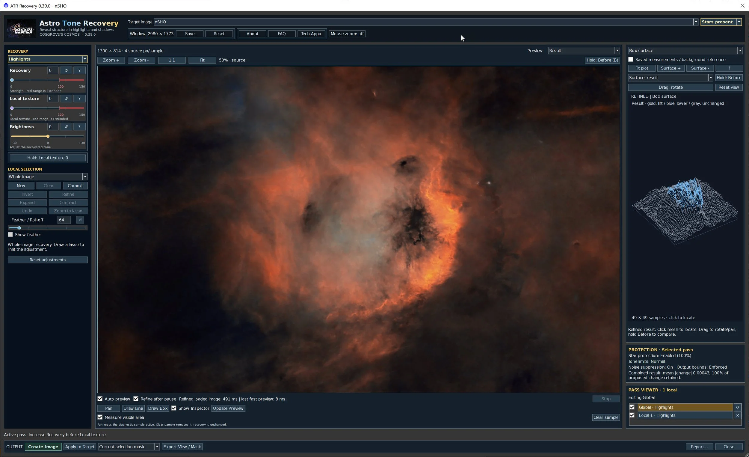
The first utility is the Astro Tone Recovery tool. This tool recovers detail lost in an image's highlights or shadows. This tool brings out detail still present in bright highlights and deep shadows by adjusting the tone scale and enhancing local structure. It cannot recover information that has been completely clipped from the source data. Can’t you just do that with the Curves Transformation tool or the HDRMT tool? Well, yes - but it’s slow and awkward. This tool is data-driven, recovering details you cannot see, changing the tone scale, and enhancing scale-level detail at the same time. It has highlight mode, dust mode, and weak signal mode. This is more automated and controlled, and you can apply it selectively using a lasso.
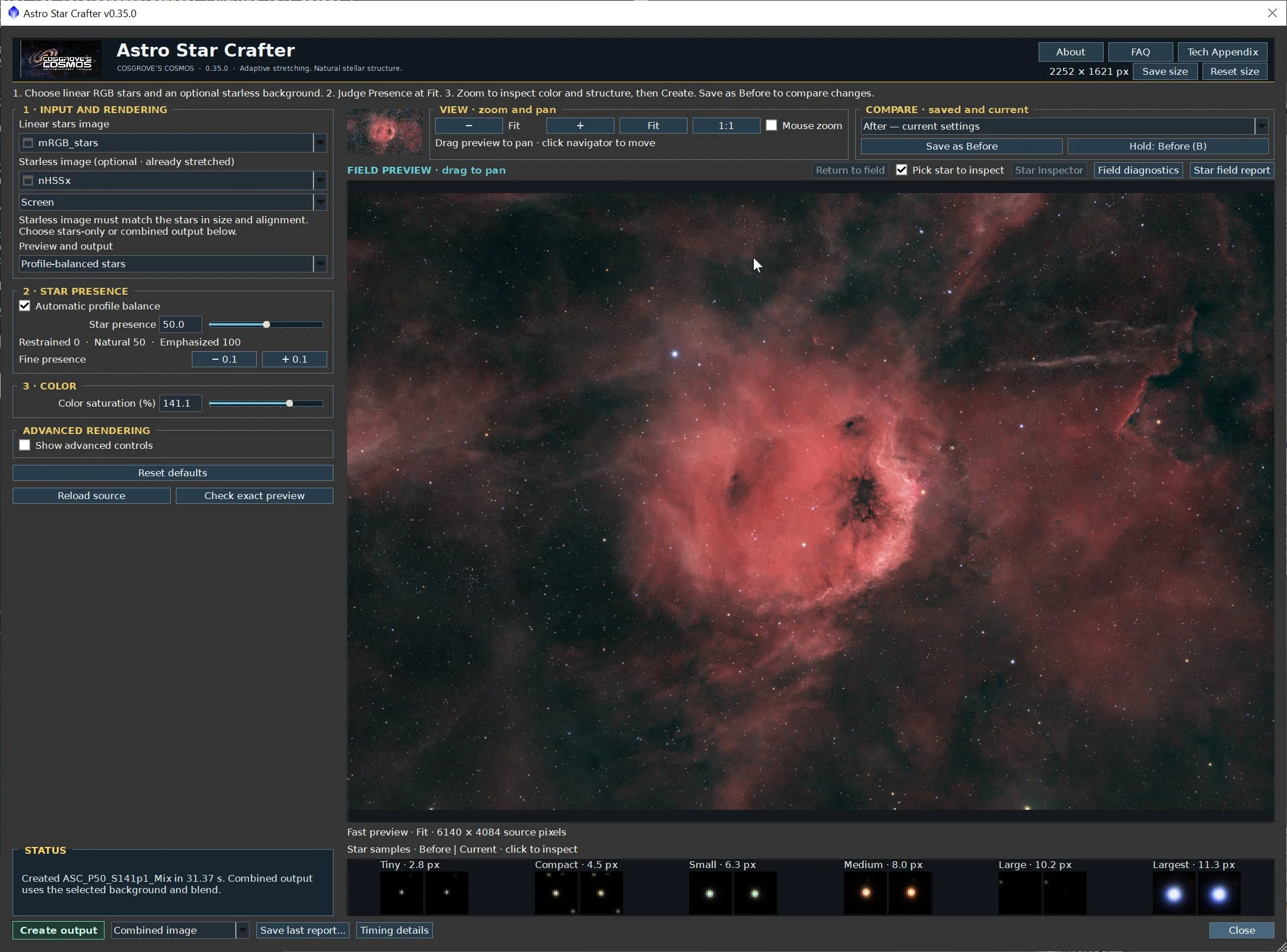
The second tool I will be using is initially called the Astro Star Carfter. This is a star-stretching and star+starless image recombination tool. This is designed for starless workflows. Many star stretchers exist, but most do their stretching based on histogram operations. I wanted something more adaptive that would drive the stretch by analyzing and preserving the structure and color of the stars. The tool suggests an initial stretch and shows you what your stars will look like. You can also add your starless image to see how the stars look with the rest of the content. Then you have two abilities. The first lets you change your star size/brightness preference, along with color saturation. The other reports on star quality, letting you inspect individual stars and see how your preference changes affect them. Then, once you have the look you want, you will combine the images and write out the new image.
Other than that, the processing was pretty straightforward.
I did have an issue: my RGB star data had very different sub-exposure times. Blue exposures were 30 seconds, while Red and Green exposures were 90 seconds. Fortunately, I had collected cal data for all of the times. But once I had master files and combined them to form the initial RGB color image, the color balance was terrible, as you might expect. DBE substantially improved the background balance, and SPCC subsequently calibrated the stellar colors.
So for this project I processed the starless SHO and HSS images in parallel. Once I got them to a reasonable nonlinear position, I did a comparison you can see below.
The initial HSS version (click to enlarge)
The initial SHO versio of the image. (click to enlarge)
I liked both, but I was drawn more to the SHO version because it had a richer, more balanced color palette.
I shared it with my local group of Astrophotography friends, and they all liked the SHO version better, so I decided to complete and go with that image.
Detailed and Annotated Image Processing Walkthrough
Typically, I conclude one of these imaging projects by documenting the processing steps I used on this image. But this section can make the overall post very large and, at times, slow to load.
I am now creating a secondary, standalone page to hold this information. You can access this page by clicking the link below. To return to this page, click the back arrow in your browser or select a different menu option at the top of the page.
I hope you like this new format!
Use the link below to view the detailed image-processing walkthrough for this imaging project.
SH2-173 Detail Processing Page
Final Results
I find this image intriguing for several reasons. First, I SEE a dog's face, not the Phantom’s Mask. I can see the mask if I try hard, but to me it's a friendly puppy hanging out in space.
While this is an SHO image, the final colors are softer and more muted than many SHO images, and I like that difference as well.
Sometimes space images strike me as being cold and brash at the same time. This one gives me a very differnt vibe and I like having that in my portfolio.
I would be very interested in your thoughts as well.
More Info
🔭 Target & Location
The Phantom of the Opera Nebula — Anthony Ayiomamitis
An astrophotographic presentation of Sh2-173 with its sky position, an explanation of the mask-inspired nickname, and equipment and exposure details for an H-alpha and broadband image.
Cassiopeia — Constellation Guide
A guide to the Phantom’s home constellation, including its familiar W-shaped star pattern, the star Caph, mythology, and other notable deep-sky objects.
📜 History & Catalog Background
The Sharpless Catalog & Observing Guide — Reiner Vogel
An observer’s introduction to Stewart Sharpless’s catalog, its origins in photographic sky surveys, and the classification of its nebulae. Includes access to an observing atlas with images and finder charts.
🔬 Science & Observations
Decoding Nebulae — NASA Science
An accessible explanation of emission, reflection, and dark nebulae, with examples showing how gas, dust, and young stars shape their appearance. General background for understanding the structures seen in Sh2-173.
Unveiling the Birth and Evolution of Sh2-173 — Cichowolski and Colleagues
The principal research study used for this project’s science discussion. Combines optical, radio, and infrared observations to investigate the ionizing star, surrounding gas and dust, young-star candidates, and possible triggered star formation. The page provides a summary and access to the full paper.
📸 Imaging & Narrowband Color
Sh2-173 in H-alpha and RGB — AstroKin
An imaging example with separate H-alpha and RGB views, acquisition details, a finder chart, and an annotated image. Useful for comparing how narrowband and broadband exposures reveal this faint target.
A Perfect Storm of Turbulent Gases — ESA/Hubble
A striking example of the SHO color palette, mapping sulfur to red, hydrogen to green, and oxygen to blue. This feature depicts Messier 17 rather than Sh2-173 and explains how stellar radiation sculpts glowing gas.
Imaging Platform Used
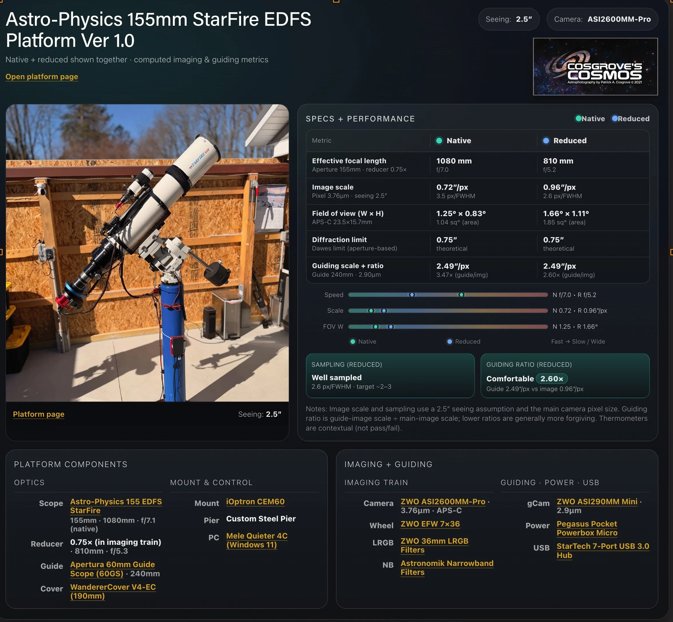
The details for the AP155 Platform.
Platform used for this project
Software
Capture Software: PHD2 Guider, NINA
Image Processing: PixInsight, Photoshop - assisted by Coffee, extensive processing indecision and second-guessing, editor regret, and much swearing…