
Sh2-54 - The Serpent Nebula - 8.9 Hours of SHO
Date: June 28, 2025
Cosgrove’s Cosmos Catalog ➤#0140

My SHO image of the region around SH2-54. (click on the image for a high res view via Astrobin.com)
Published in Orbital Today - Jul 3, 2025!

Click to go to webpage!
Published in BBC Sky @ Night - October 2025!


Table of Contents Show (Click on lines to navigate)
Preface
Of course, everyone knows that when you get a new telescope or camera, you are likely to experience several weeks of cloudy weather that will prevent its use.
With the completion of my Whispering Skies Observatory and the purchase of a new galaxy scope platform, I was certain that I would not see a clear sky for a year.
It has been bad, but I did have two clear nights in late April, and we just had another couple of days on June 22nd and 23rd with no Moon, no clouds, and minimal smoke! This was the first image I chose to process from those nights!
About the Target
Sharpless 2-54, also known as RCW 167, Gum 84, and W35, is located in the tail of the constellation Serpens about 6,000 light-years from Earth.
Sh2-54 is a giant H II region roughly 140′ (2.3°) across. It glows in H-alpha where radiation from dozens of O- and B-type stars ionises the parent molecular cloud. Infra-red and radio surveys have catalogued hundreds of embedded young stellar objects; a well-studied example is the high-mass protostar IRAS 18151-1208, whose collimated molecular jets trace ongoing massive star formation.
The nebula was entered in Stewart Sharpless’s 1959 catalogue of emission regions and is now a benchmark field for studying the early lives of massive stars.
Also in the field is NGC 6604, also known as Cr 373. The bright open cluster can be seen towards the lower right side of the image.
Discovered by William Herschel in 1784, it lies 4,600–5,500 light-years away and is only 4–6 million years old. Its dozen or so O-type stars provide most of the UV flux that lights up Sh2-54, while their powerful winds sculpt cavities and trigger secondary star-formation along the nebular edges. NGC 6604 is the densest concentration within the Serpens OB2 association and sits ∼210 light-years above the Galactic plane, giving observers a relatively unobscured view in visible light.
The central cluster NGC 6604 inside Sh 2-54 hosts two of the ~20 known “particle-accelerating colliding-wind binaries”—HD 167971 and HD 168112. The supersonic winds from their massive O-type components slam together, creating shock fronts that boost electrons to relativistic speeds and produce detectable hard X-rays and non-thermal synchrotron radio emission. Recent milliarcsecond-resolution VLBI images resolved the curved shock zone itself, confirming the nebula as a natural laboratory for cosmic-ray physics. 
A Little About the Constellation
Serpens is the only modern constellation that is non-contiguous: its western half, Serpens Caput (the Head of the snake), lies west of Ophiuchus, while Serpens Cauda (the Tail) stretches east and south of the same figure. SH2-54 is found in this later section. Separating them is the constellation Ophiuchus - the Snake Bearer!

Serpens Cauda on the left, Serpens Caput towards the right, with Ophiuchus in the center! (: https://www.go-astronomy.com/constellations.php?Name=Serpens)
First catalogued by Ptolemy in the 2nd century CE, it remains part of the IAU’s official list. With the Milky Way running through its tail, Serpens offers a mix of star-forming regions (Sh 2-54, M 16), globular clusters (M 5), and exotic galaxies such as Hoag’s Object. Observers at mid-northern latitudes see the head high in the south on June evenings and the tail—home to your image target—well-placed from July into early September.
Part of a larger complex
Sh2-54, the Eagle Nebula (M 16), and the Omega Nebula (M 17) all belong to the same giant molecular complex in the Sagittarius spiral arm. Comparing these neighbouring objects lets astronomers trace different evolutionary stages of OB-cluster formation within a single cloud. The ESO VLT Survey Telescope released a 3-gigapixel wide-field in 2023 that mosaics all three regions, highlighting the filamentary gas, dust pillars, and feedback-driven bubbles they share.

Two of the sky’s more famous residents share the stage with a lesser-known neighbour in this enormous three-gigapixel image from ESO’s VLT Survey Telescope (VST). On the right lies the faint, glowing cloud of gas called Sharpless 2-54, the iconic Eagle Nebula (Messier 16) is in the centre, and the Omega Nebula (Messier 17) to the left. This cosmic trio makes up just a portion of a vast complex of gas and dust within which new stars are springing to life and illuminating their surroundings.
Credit: ESO
Why it matters
Star-formation laboratory: High protostar density plus a still-young massive cluster give researchers a snapshot of both early and slightly later stages of stellar evolution.
Feedback studies: The interaction between NGC 6604’s winds and the surrounding gas helps test models of triggered star formation and bubble expansion.
Kinematics: Gaia DR3 proper-motions are refining membership of the Serpens OB2 group and mapping how the cluster and gas are moving through the Milky Way.
The Annotated Image

Created in Pixinsight using the ImageSolver and AnnotateImage scripts.
The Location in the Sky

This annotated image created with Imagesolver and FInderChart Scripts in Pixinsight.
About the Project
Picking the Target
During my last clear night, which was in April, we were still in Galaxy season. At that time, I decided to choose a set of galaxy clusters as my targets. That was great to get things going, but in truth, I missed shooting narrowband images with more structure and drama.
When the next clear night came along, we were in June, and I started searching for something that would catch my eye.
I often search through various catalogs for ideas. One of my favorites is the Sharpless catalog. As I thumbed through its objects, I came across SH2-54. I had never seen this target before, and I was very intrigued. The area was a rich H-II region with some dark and dusty regions as well. The bright region seemed to have a lot of structure and detail, and I really wanted to try my hand at capturing this!

Data Collection
The weather cooperated on June 22nd and 23rd. These were surprisingly hot days for June, with temperatures ranging from the high 80s to the low 90s. Because of this, I opened the observatory around 8 pm to let things cool down.
The nights are very short right now, so I did my best to maximize my capture time. I only had about 4.5 hours of astronomical darkness, so I think I did well to capture 8.9 hours of data on these two nights.
Because the temperatures were running very high during the day, I knew that my camera coolers would be straining to hit my typical aim temps of -15C. Because of this, I decided to run at -10 C for this session.
And because I was shooting narrowband, I set the ASi2600MM-Pro camera gain to 100.
I did not quite realize it at the time, but the hot weather seemed to create a problem that I was as yet unaware of. Apparently, the heat caused the metal on the scope to expand, and this loosened the connection between the camera and the camera rotator!
I had a hint of this when NINA ran the Slew, Center, and Rotate routine.
It seems to take a lot of tries to get the rotation nailed down. Usually, three attempts are all it really needs. However, this time it took about six attempts, which I found odd.
The reason for this is that the camera was also unscrewing from the rotator as the rotator was turning things!
Other than this, things were well behaved, and I seemed to enjoy excellent tracking.
After the second night, I used the third night to shoot calibration frames. When I was attaching my Flat Light source, I noticed that the camera was loose on the rig. I was very careful not to rotate things from their original position, as I wanted the Flats to capture the correct rotation angle; however, it got there. If I screwed the camera back in, it would no longer track what was used when the subs were captured.
Reviewing the Data
I always blink all of my data before doing any processing. When I did that this time, I saw something unusual. I saw circular star trails!
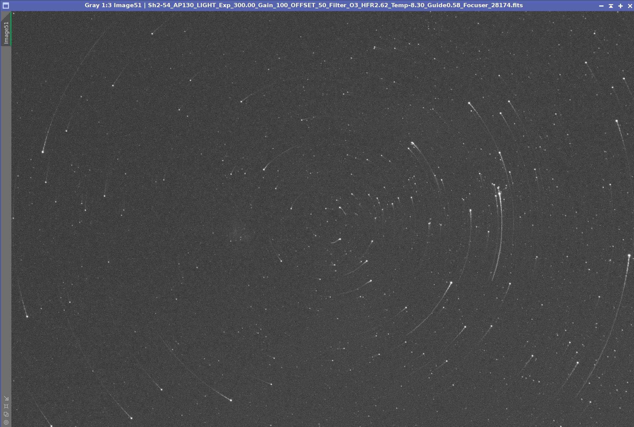
The Strange Rotational Trails I saw….
That one was a new one on me!
I only saw a couple like this, but I realized that the camera must have self-rotated during the sub to produce this. I also noticed that some of the images were slightly rotated in relation to one another. This was a problem with the loose camera again!
I figured that registration would correct for this, but I was expecting my flat calibration to be a little odd this time.
Processing Overview
Due to the rotation, I decided it would be best to perform DBE on each master image before combining them. This was done in the hope of addressing any residual flat calibration issues that might arise from the rotation on some frames.
With this one change, I used by normal narrowband workflow that looks like this from a high level:

The high level SHO workflow used.
Two other aspects should be raised about the processing approach I used for this project.
I used the NarrowbandNormalization script to process the colors on the initial color image and on the stars-only images to get the color I wanted. In the past, I typically did this by hand, but I wanted to explore the use of some new (to me ) tools. This seemed to work well, and the preview capability was appreciated.
The second is the use of the SelectiveColorCorrecion script instead of using my standard color masking techniques.
I liked using each tool and may consider using them as my standard method as I move forward.
Look below for the complete step-by-step processing walkthrough! Note: This walkthrough is based on Pixinsight.
Final Results
The final image captures an interesting and unusual field in Serpens that I don’t think is imaged all that much.
After posting it, I received several comments mentioning that the bright area is often perceived as a spooky face. I had not seen any reference to this when working on the image, but if you take the close-up here and squint just right, you might see that!

Can you see a face?
I think having a lot more integration time would have been advantageous. Not just for the better SNR that would result, but because it would let me cull the less sharp images and enhance the sharpness of the whole scene.
What did you think about it?
More Information
📖 Background & Overview
Sh 2-54 — Wikipedia – Concise encyclopedic entry listing designations (RCW 167, Gum 84, W35), size, distance ≈ 6 200 ly and discovery by Stewart Sharpless in 1959.
NGC 6604 — Wikipedia – Summary of the 6 Myr-old OB cluster that powers Sh 2-54, with distance, stellar content and historical notes from William Herschel’s 1784 discovery.
🔬 Research & Data
“Magnetic ‘Rivers’ Feed Young Stars” – NASA – SOFIA polarimetry showing magnetic filaments funnelling gas into the Serpens South nursery inside Sh 2-54.
High-Resolution Radio Imaging of HD 167971 & HD 168112 – arXiv (2024) – VLBI study of two particle-accelerating colliding-wind binaries in NGC 6604, probing shock physics.
The Long-Period Orbit of the Particle Accelerator HD 167971 – arXiv (2012) – X-ray/optical analysis of NGC 6604’s brightest massive system and its hard-X-ray emission.
🖼️ Images & Media
Sh 2-54 Visible Mosaic – ESO VST (eso2301b) – 17 k-pixel H-α panorama revealing dust lanes and ionised gas.
Sh 2-54 Infrared vs Visible Slider – ESO VISTA/VST (eso2301a) – Side-by-side view showing how IR light penetrates dust.
Serpens South Protostars – Spitzer – IR image of 50 protostars embedded in Sh 2-54.
Star Cluster NGC 6604 – ESO WFI (eso1218a) – High-resolution optical image of the OB cluster and surrounding nebula.
Wide-Field DSS Panorama around NGC 6604 – ESO (eso1218c) – 3-degree locator chart for amateur fields.
🛰️ Space-Telescope Context
VST 3-Gigapixel Mosaic of Sh 2-54, Eagle & Omega Nebulae (eso1719a) – Places Sh 2-54 alongside its famous neighbours within the same giant molecular complex.
(No full-field Hubble or JWST images of Sh 2-54 exist; its angular size far exceeds their cameras. Use the cluster and IR assets above instead.)
🌟 Popular Articles & Press
“Dazzling Photo Reveals Bright Young Star Cluster Inside Cosmic Clouds” – Space.com – Accessible description of ESO imagery and star-formation feedback in NGC 6604.
“A Cluster within a Cluster” – Astronomy Magazine – Historical context and observational tips for NGC 6604 and Sh 2-54
Capture Details
Lights Frames
Taken the nights of June 22nd and 23rd, 2025
36 x 300 seconds, bin 1x1 @ -10C, Gain 100, Astronomiks 6nm Ha - 36mm unmounted
35 x 300 seconds, bin 1x1 @ -10C, Gain 100, Astronomiks 6nm O3 - 36mm unmounted
36 x 300 seconds, bin 1x1 @ -10C, Gain 100, Astronomiks 6nm S2 - 36mm unmounted
Total - after culling bad subs - of 8 hours and 55 minutes.
Cal Frames
25 Darks at 90 seconds, bin 1x1, -10C, gain 100
30 Dark Flats at Flat exposure times, bin 1x1, -10C, gain 100
One set of Flats done:
15 Lum Flats
15 R Flats
15 G Flats
15 B Flats
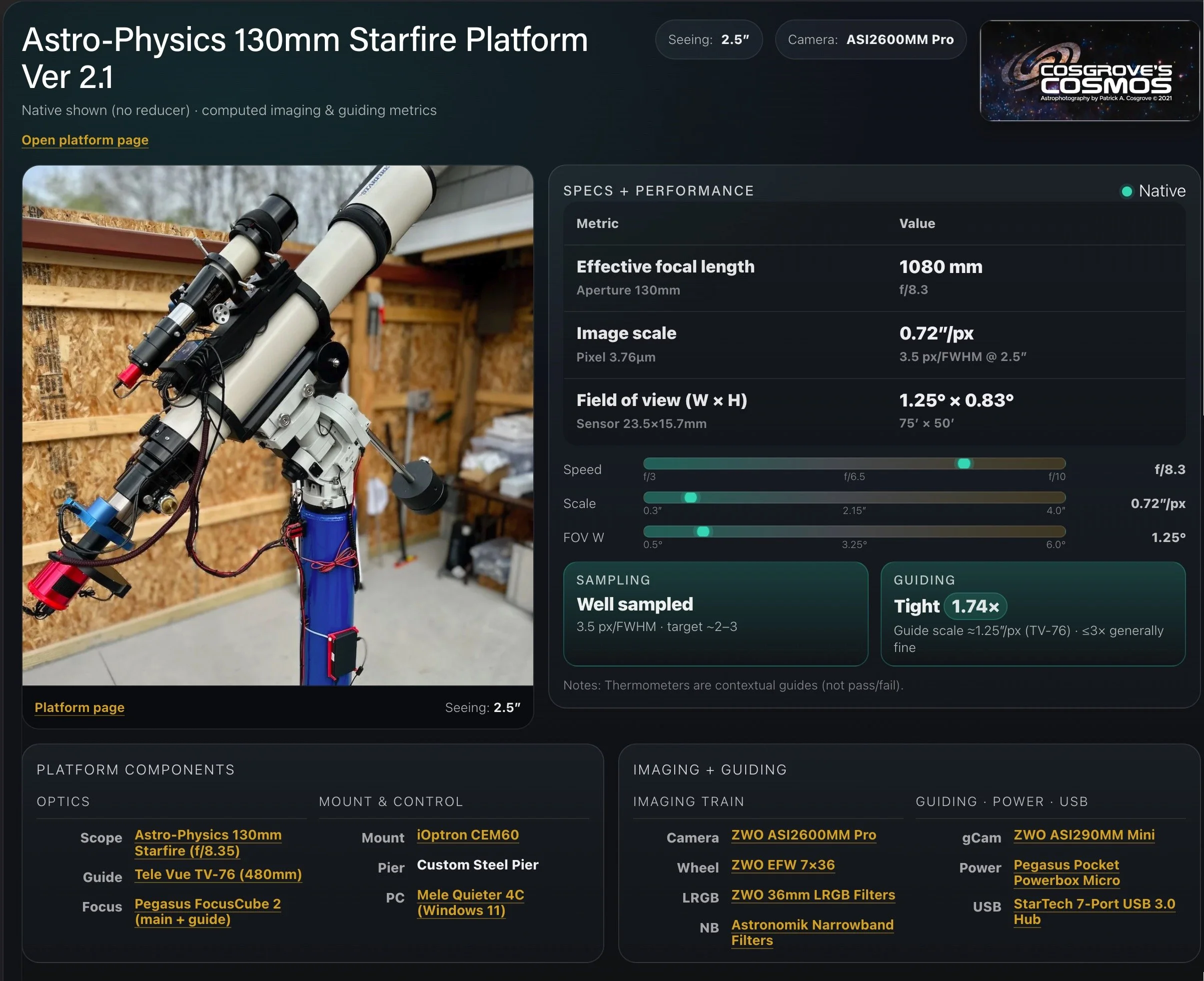
Platform used for this project
Software
Capture Software: PHD2 Guider, NINA
Image Processing: Pixinsight, Photoshop - assisted by Coffee, extensive processing indecision and second-guessing, editor regret and much swearing…..
Image Processing Walkthrough
(All Processing is done in Pixinsight, with some final touches done in Photoshop)
1. Blink
Ha
One frame with rotation trails from the loose camera removed
One other seemed to have a different rotation than the other frames, but I left it.
O3
1 rotation frame removed
1 sub masked by thin clouds removed
Some trails
S2
One trasiled rotation removed
Others are rotated - not sure what that will mean
Darks
All looks ok
Dark Flats
All looks ok
Flats
all good
2. WBPP 2.8.8
Reset everything
Load all lights
Load all flats
Load all darks
Select - maximum quality
Reference Image - auto - the default
Select the output directory to wbpp folder
Enable CC for all light frames
Pedestal value - auto
Darks -set exposure tolerance to 0
Lights - set exposure tolerance to 0
Lights - all set except for linear defect
set for Autocrop
Set for 2X Drizzle
Executed in 3:54 minutes - no error!

WBPP Calibration View

WBPP Post Calibration View

WBPP Pipeline View
3. Load Master Images
Load all master images and rename them.

Master Ha, O3, and S2 images
4. Iniital Process of Linear Narrowband data
For each filter, run DBE. Sample patterns were customized to handle the weird non-uniformities I saw due to the loose connection.
Create the initial SHO Image by using the ChannelCombination Tool
Run the NarrowbandNormailzation Script. See parameters used below.
Invert the image so we can remove the residual magentas seen
Run SCNR Green at 1.0
Do a final image invert
Run PFSImage to measure star sizes X= 3,.4, Y= 3.76
Run BXT Correct Only
Run BXT Full with the parameters listed below. A little more aggressive than what PFSIMage suggested.
Run NXT V3 with parameters documented below.
Run STX with large sample size to create a starless and Stars only image.
Master Ha Sample Pattern (click to enlarge)
Master O3 Sample pattern (click to enlarge)
Master S2 Sample Pattern (click to enlarge)
Master Ha Before DBE (click to enlarge)
Maser O3 Before DBE (click to enlarge)
Master S2 Before DBE (click to enlarge)
Master Ha after DBE (click to enlarge)
Master O3 After DBE (click to enlarge)
Master S2 After DBE (click to enlarge)
Master Ha Background
Master O3 Background (click to enlarge)
Master S2 Background (click to enlage)
The inital SHO Image (click to enlarge)

Params used in NarrowbandNormailization
After SCNR Green 1.0 (click to enlarge)
After Narrowband Neutralization (clikc to enlarge)
Invert the image. (click to enlarge)
After Final Invert (click to enlarge)

PFSImage Results

BXT Parameters used.

NXT Parameters used.


Master SHO before BXT Correct Only, After BXT Correct Only, After BXT Full, After NXT V3

Final Linaer SHO image.
Stars-only after running STX (click to enlarge)
Master RGB Starless Image after running STX (click to enlarge)
5. Process the SHO Starless Image
Normally, the first thing I do with a nonlinear starless image is to adjust the tone scale and color saturation with CT, and then I start creating color masks, so I do targeted color enhancements. For this image, I decided to try the Selective Color Correction script. With this tool, you can do several corrections, one after another, and a preview shows you the results as you make changes. It actually creates color masks in the background and then applies the changes you make. It will also let you preview the mask being made, so you can fine-tune things there as well. It seemed to work okay, but I did kind of miss creating my own masks manually.
I did three interactions, which I will discuss below, and then show the results and progression further down the page.
For the first iteration, I was working on the yellow colors. I boosted the yellow and then adjusted the saturations and luminace

Yellow adjustment paramaters.
In the next iteration, I was working on the blues. Boosting both blue and cyan and satiation while backing off the luminance.

Blue adjustment parameters.
Finally, I worked on the red - boosting yellow and reds.

Red Adjustments.
Apply NXT - see the NXT Panel snap below.
Run MLT Shaprening with the panel values shown below.
Create Mask_1 using GAME to focus on the bright feature in the upper left.
Apply Mask_1
Adjust CT with the mask
Run HDRMT with levels = 6 to bring detail out in the highlights
Run Unsharp Mask params from the screen snap below
Run MLT Sharpening with the params shown below.
Remove the mask
Create Mask_2 with the GAME script to work on the right side of the image
apply Mask_2
Apply CT
Create Yellow_Mask using Bill Blanshan’s scripts
Apply the Yellow_Mask
Apply CT
Remove the mask
Run the DarkStructure Enhance script using the default params.
The initial SHO Starless image (click to enlarge)
After the second SCC adjustment for blues (click to enlarge)

NXT V3 params used for the next step.

MLT Params used for the sharpen operation
After the 1st SCC Adjustment for yellows (click to enlarge)
After 3rd SCC Adjustment for reds (click to enlarge)
After NXT V3 (click to enlarge)

After MLT Sharpening done using an interior mask (click to enlarge)
Mask_1 created with the GAME script (click to enlarge)
Mask_1 in place. (click to enlarge)
After CT with Mask_1 (click to enlarge)

UnsharpMask params used below with Mask_1 below.

MLT Sharpening used with Mask_1 below.


Before HDRMT, After HDRMT, After Unsharp Mask, and After MPT Sharpening.
Mask_2 taretign the right side of the image.
Ct with Mask_2. (click to enlarge)
Yellow Mask - created with Bill Blanshan’s Script.
CT with Yellow_mask (click to enlarge)
6. Process the Star Images
Take the linear stars-only image from the STX run and use NarrowbandNormalization to clean up some of the unusual narrowband colors. This is mostly SCNR for green. I experimented with other params, but I thought these were the best.
Then I used the HostogramTransform process to go nonlinear, bring out star sizes I thought looked best.
Finally, I did a CT to clean up colors, saturations, and some tone scale to finalize the stars I would use. I liked the final result.
Linear Stars from STX - the starting point! (click to enlarge)
Linear stars after NarrowbandNormalization (click to enlarge)

The paramters used to clean up the stars a bit.
Initial Nonlinear Stars (click to enlarge)
Nonlinear stars after NarrowbandNormalization (click to enlarge)
Zoomed in version of the final stars - some warm and cool stars without the wierd greens and magenta tones that NB stars can have. (click to enlarge)
7. Add The Stars Back In
Use the ScreenStars Script to add the stars back in.
The SHO Stars Image (click to enlarge)
The Final Starless SHO image (click to enlarge)

ScreenStars Panel.

The image with Stars inserted!
8. Export the Image to Photoshop for Polishing
I am pretty happy with the image and ready to polish it in Photoshop.
Save the image as a TIFF 16-bit unsigned and move to Photoshop
Make final global adjustments with Clarify, Curves, and the Color Mixer
Select some feature areas with a lasso with a 100-pixel feather, and use clarity to tweak selected detail areas.
I did a very slight crop to frame things better.
Added Watermarks
Export Clear, Watermarked, and Web-sized jpegs.

The Final Image!