
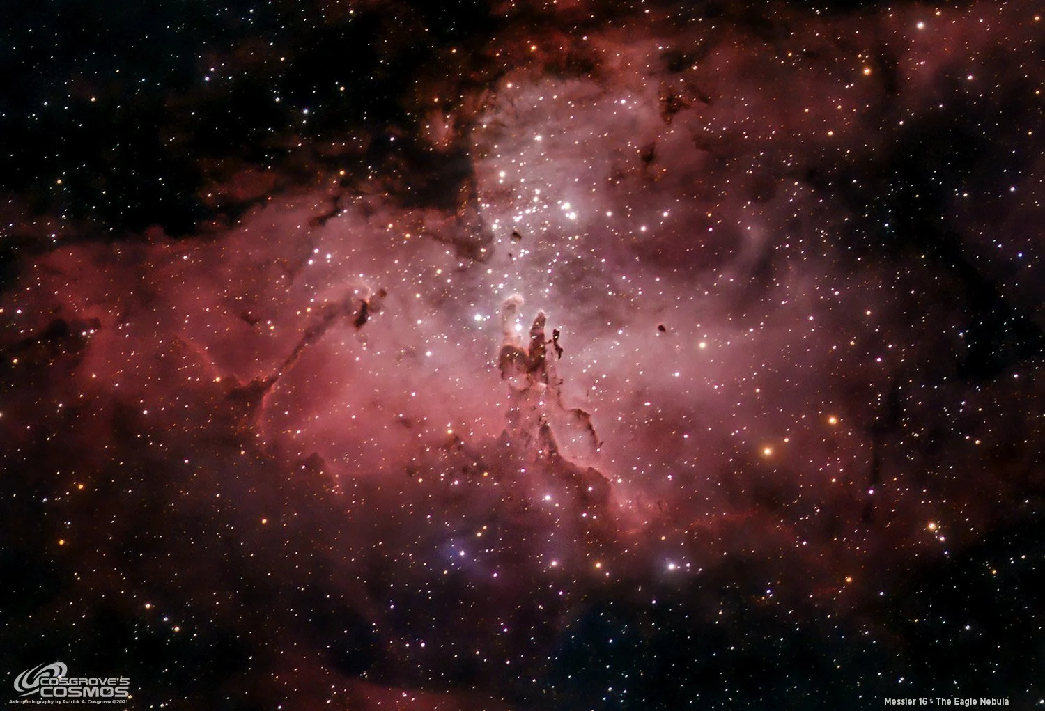
Messier 16 - The Eagle Nebula/The Pillars of Creation, 4.75 hours in SHO (A Narrowband Test of the SCA260 Scope)
Date: July 10, 2025
Updated 8-13-25
Updated 7-30-25 based on feedback on the SXT issue from Russ Croman
Cosgrove’s Cosmos Catalog ➤#0141

First narrowband test image for the Sharpstar SCA260 V2 and the Whispering Skies Observatory! (click for access to full res image via Astrobin.com)
Granted “Explore” Status on Flickr on 7-13-25!

Table of Contents Show (Click on lines to navigate)
Background
We’ve had a few clear nights, and on one of those, I wanted to do a quick test with my new Sharpstar SCA240 V2 scope on a bright narrowband target. This was seen as a quick test.
So I collected one night of data on Messier 16 to see how things were looking. It turned out to be both an interesting and challenging image. as you will see….
About the Target
Overview
Messier 16—better known as the Eagle Nebula—is located some 6,500 light-years away in the northern reaches of the constellation Serpens Cauda. What the eye sees as a modest sixth-magnitude patch is actually a large H II region, its hydrogen set aglow by the ultraviolet output of the young open cluster NGC 6611 at its heart. Among the sculpted ridges and voids rise the famous “Pillars of Creation,” three dust columns roughly four to five light-years long that silhouette against the cavity they helped carve.
Anatomy of a Stellar Nursery
Note: NGC 6611 is not shown in my annotated image as the label conflicts with the M16 label. However, NGC 6611 is an open star cluster that can be seen behind and around the M16 label.
NGC 6611 is barely one to two million years old, yet already hosts dozens of O- and B-type giants whose radiation and stellar winds both erode and ignite the surrounding cloud. At the pillars’ tips lie evaporating gaseous globules (EGGs): dense knots in which protostars continue to accrete even as their cocoons boil away. High-resolution imaging shows shear flows, shock fronts, and infant stars in the infrared that are invisible at optical wavelengths. Models and recent time-lapse analyses suggest the columns will survive another hundred thousand years or so—long by human reckoning, fleeting by galactic standards.
A Brief History of Discovery
Swiss observer Jean-Philippe de Chéseaux first noted the nebula in 1745-46; Charles Messier added it to his catalog in 1764. It remained an obscure binocular object until Hubble’s 1995 Wide Field and Planetary Camera 2 portrait catapulted the “Pillars of Creation” into pop-astronomy fame. Hubble’s 2014 revisit sharpened the view, Herschel and Spitzer pierced the dust in the far-infrared, and in 2022, the James Webb Space Telescope’s NIRCam and MIRI instruments revealed thousands of newborn stars embedded inside the very figures that Hubble made famous.
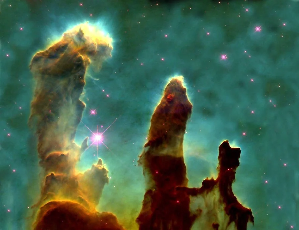
1995 — Hubble WFPC2 (visible-light original)
Credit: NASA, ESA, STScI, J. Hester & P. Scowen (Arizona State University)

2014 — Hubble WFC3/UVIS (visible-light high-definition revisit)
Credit: NASA / ESA / Hubble Heritage Team (STScI/AURA)
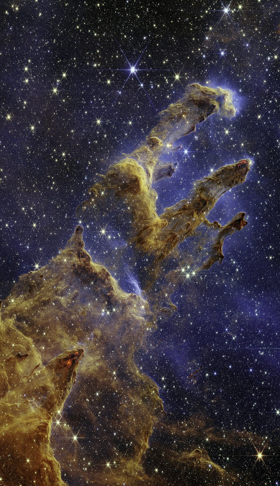
2022 — JWST NIRCam (near-infrared view)
Credit: NASA / ESA / CSA / STScI — image processing by J. DePasquale, A. Koekemoer & A. Pagan (STScI)
Looking Ahead
Although the pillars are slowly photo-evaporating, they will continue producing new stars for tens of thousands of years before finally dispersing into the wider Sagittarius spiral arm. From Earth’s vantage point, however, their present-day grandeur is safely “time-locked”: even if a supernova has already shattered the columns, that light will not reach us for many human lifetimes.
Annotated Image
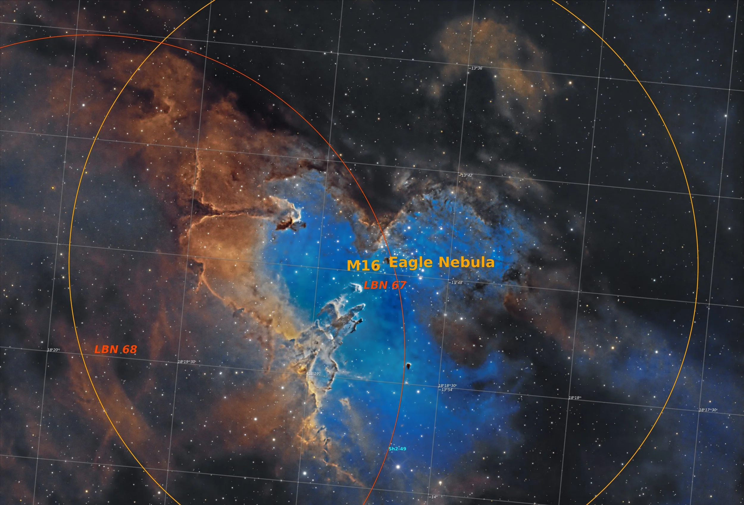
Image created with Pixinsight’s ImageSolver and AnnotateImage scripts.
Location in the Sky
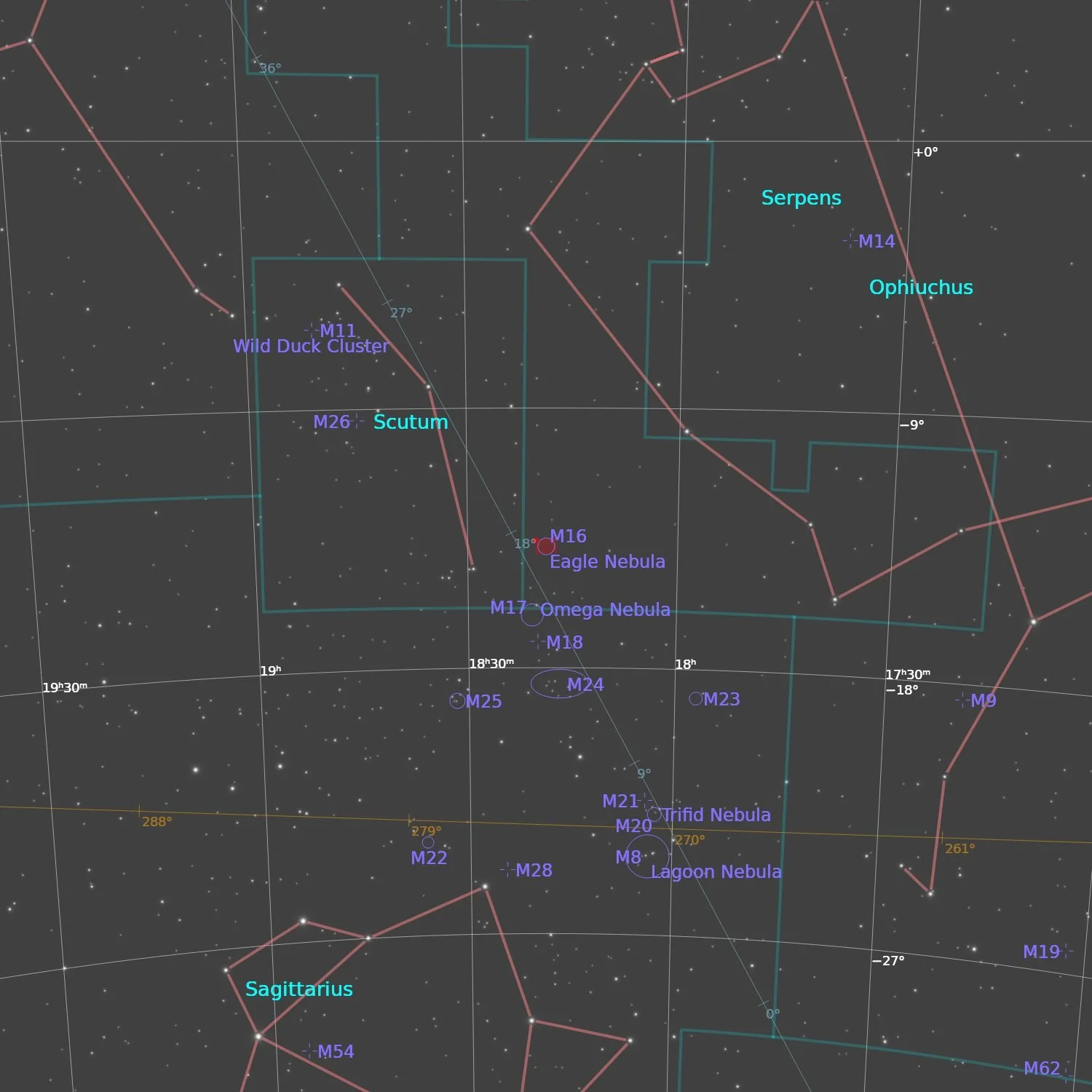
Findershart created with Pixinsight’s ImageSolver and FinderChart scripts.
About the Project
This is actually my third imaging project on the Snew C260 scope. I have not yet documented the second because I was disappointed with the framing I did, which made the project kind of blah. However, I document and share even my failed projects, so I will eventually get this done.
After having a less-than-thrilling reaction to project number 2, and knowing that the moon was soon to return, I decided to use the night of June 26 to complete this little project.
It was meant to be a test since I knew I would only get one night of data from it. But I was eager to do a narrowband test and see how the scope did.
I set up NINA to pursue M16, and the entire night’s sequence ran smoothly with no major issues. Very simple. Very easy.
The fact that I got 4.75 hours of good data on such a short note shows that things went well!
Previous Efforts
First Attempt: I first shot M16 back in August of 2019. It was one of my first images - and it really looks that way! This was shot on my Williams Optics FLT 132mm with an OSC camera with a grand total of 0.3 hours!! See that imaging project HERE.
Second Attempt: June 2020. Same telescope and camera. 2.6 hours Integration. Much better! See that Project HERE.
Third Attempt: July of 2021. This was shot with my Astro-Physics 130 platform, in narrowband. 3.9 hours of integration. This is one of my favorite images. This current image has more color and detail, but I still like this one the best! See it HERE.
My 2019 Effort
My 2020 effort

My 2021 effort
This is the kind of series that an astrophotographer likes to show. A nice progression of images getting better over time.
This new image is very interesting and very good on several levels. But does it continue the progression? Is it significantly better than the last one? I would say it is different, but not necessarily better.
Why would this be?
Maybe I am just used to the older one and more attached to it
I came from my Astro-Pysics scope, which has amazing sharpness and contrast. The new one is with a Super Cassigrain - it is good but the quality of the optics will be different.
Maybe the nights I shot the old one were better! It was very hot and humid when the most recent was shot and maybe the skies were just not as transparent.
Data Capture
We had a string of 3 clear nights, and on the third night, June 26, I decided to shift targets and do this narrowband test.
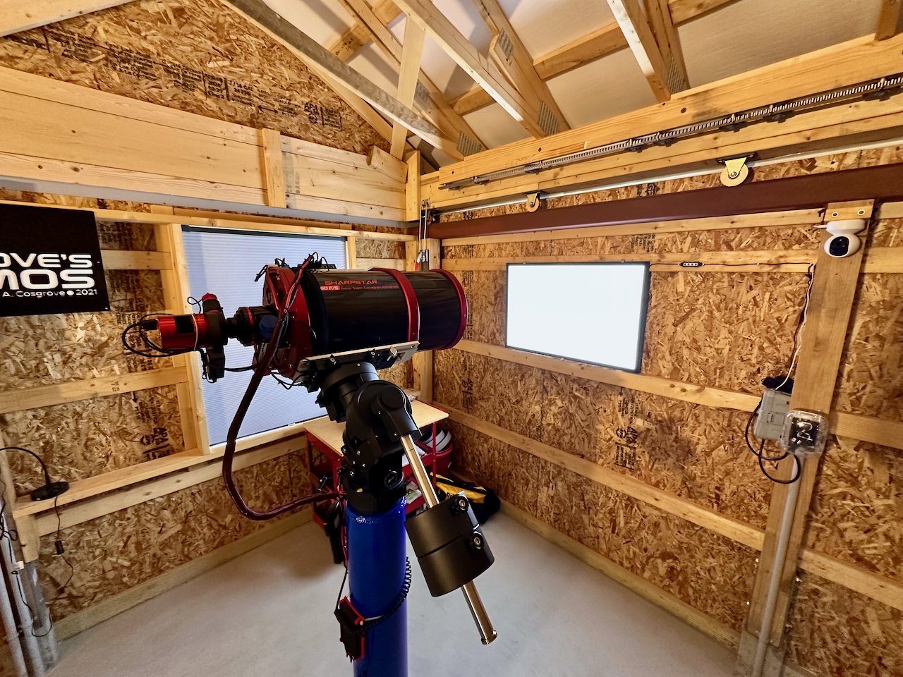
My Flats set up for the SCA260.
For this project, I used the SharpStar SCA260 V2, pairing it with the ZWO ASI2600MM-Pro through Hα, O III, and S II filters. Over 4.75 total hours of integration.
Since I was using narrowband filters, I ran the camera with a gain of 100 and an offset of 50.
Because of the high heat, I used a target cooling temp of -10C. I was able to achieve this temp with some difficulty due ot how warm it was out.
I used my Off-Axis guider for these exposures.
All were captured on one night.
Dark and flats were captured the following night. I found that I have a light leak somewhere in my optical chain, so now I do my darks when it is actually dark out, and this solves the problem.
My flats were shot using a large LED panel mounted on the wall. I placed fans underneath, pointing up, to keep the bugs off the panel during the Flats Wizard operation.
Image Processing
The image processing for this image was more difficult than I expected.
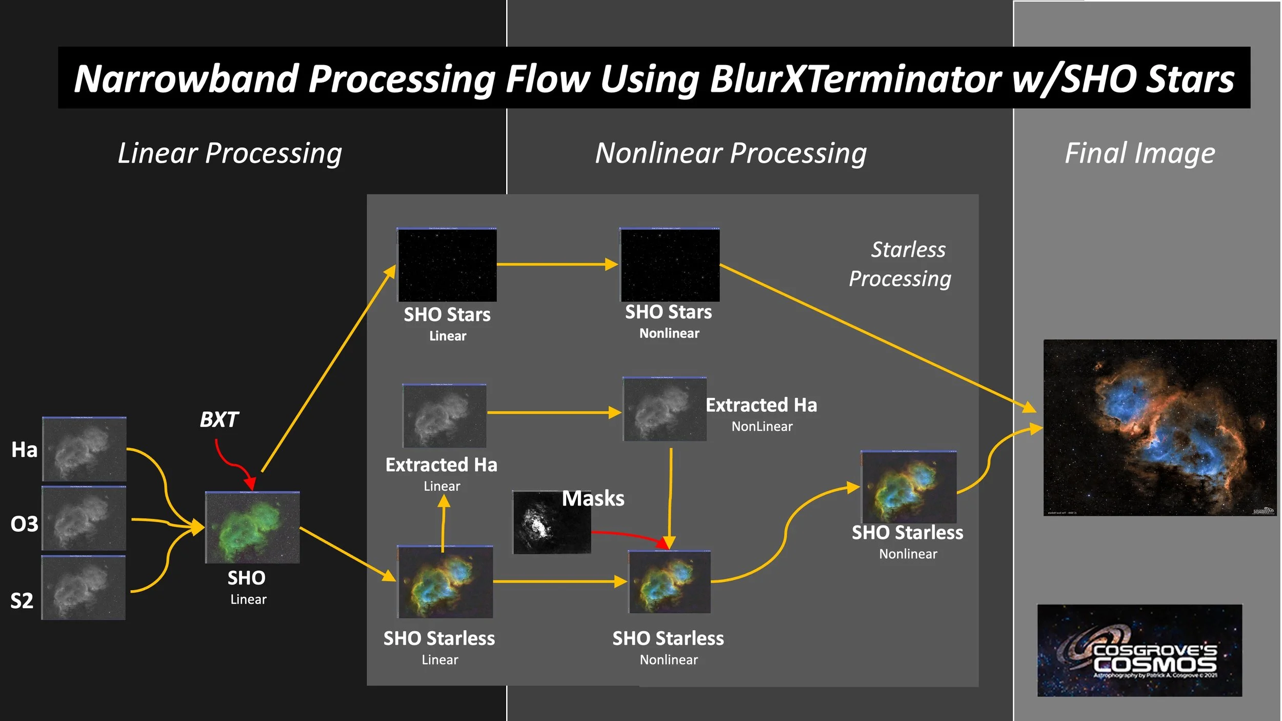
I followed my normal narrowband workflow which looks like this:
I used a drizzle 2x process on this to maximize resolution and detail.
But as I progressed, I realized that I had a problem.
In the past, I was always reluctant to switch to a pure starless workflow because the tools at the time removed stars but often left residual blemishes from the stars in the starless image. If you then stretched and enhanced the starless data, these blemishes became ugly artifacts. So, what you had to do was to remove the blemishes with a clone tool or something similar.
However, when RC-Astro released the current generation of StarXTerminator, I was hooked. With StarExterminator, it was rare to see blemishes.
Star Blemishes Return
So, I used my normal workflow, and as I reached a decent point with the nonlinear starless image, I did a quick ScreenStars to reunite the starless version with the stars to see how it was progressing.
At first, it looked great. Then I looked deeper. I saw this:

Some ugly artifacts around bright stars!
That’s not good! So I went back to the starless image, assuming the problem was there. It was.

Definately baked int the nonlinar Starless image.
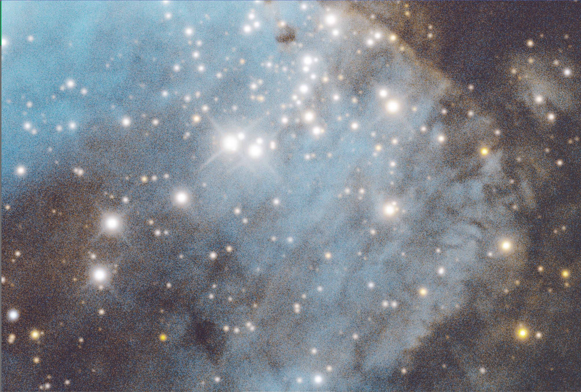
So I went back to the nonlinear master SHO image - which looked like this in a few sample spots.
Sample #1 Before StarXTerminator
Noisy, but not horrible-looking stars.
Then I applied StarXterminator. You can see faint blemishes around the location of the bright stars. But once we go nonlinear, this are amplified into artifacts that are unacceptable.

After StarXTerminator.
Here is another example. Before StarXterminator:

Sample #1 Before StarXterminator
After StartXterminator.
After StarXTerminator.
Faint - but there are definitely residual blemishes from being left by the bright stars.
Bright stars come out on the SCA260 with diffraction spikes. In general, StarXterminator does a good job with diffraction spikes. But I found that with the SCA260 and narrowband, this was not the case. Even worse, if you are aggressive with BlurXterminator, the starless results look even worse.
After going nonlinear, adding some sharpening and other enhancements, these blemishes looked much worse.
So I had to go back to square one.
I went a lot easier on BlurXterminator and stretches and I got something that looked better in the starless image:

These are much improved, but they are still there, and they looked bad when you added stars back in.
So what did I do?
I ended up exporting the final nonlinear starless images as a 16-bit TIFF file. I imported this in Photoshop and used the healing brush to eliminate them.
Here is what the image above looked like after this step:

This is much better. I only did the worst ones. If you look carefully, you can see some faint residuals that I did not bother to fix.
This produced an acceptable result, but it is not how I want my processing to go.
I will be contacting RC-Astro and asking for guidance.
Update: Some readers have suggested that a slight stretch be applied to the image before doing SXT - I will give this a try.
Major Update
〰️
Major Update 〰️
One of the things that has always impressed me with StarXterminator is how well it worked. Blemishes were rare and minimal. But these are problematic. I suspected that this had to do with the SCA260 and the nature of its defraction spikes. Perhaps they were different than what RC-Astro had trained on.
So I went to the RC-Astro website and opened a support ticket describing the problem.
I soon got a note back from Russ Croman:
Hi Patrick,
Good to hear from you, and thanks for the report.
I'm thinking that the strong diffraction rings that appear in the image (due to the large central obstruction, I am guessing) are leading to these artifacts. The current version of SXT isn't trained on PSFs of this type.
The good news is that I'm training a new version now that has a much wider range of PSF types it will support. The bad news is that this isn't available yet, and it's very difficult to say when it will be – every new version is a deep research and development project.
In the meantime, you might try applying SXT after some stretching. Preferred stretch is MTF.
Would you be willing to upload the original image for analysis and testing? I'd be happy to share anything I find, including workarounds with the current version of SXT.
Thanks,
Russ
I suspected this was the case. So I sent him three images:
The SHO image right after I did NarrowbandNormalization
The SHO image right after I applied BXT and NXT
The SHO image after running SXT
Russ quickly got back to me, asking for more details because he thought that the noise in the image looked “funky”.
As soon as he mentioned this, it got me thinking. I had just started using the NarrowbandNormalization Script. I applied before I did BXT, NXT and SXT. What if it was scaling one color a lot more than an other. That would also scale the noise differentially. I realized that could be a bad thing.
In the past, my workflow looked something like this:
LRGB:
Create RGB Image with ChannelCombination
DBE
BlurXterminator - Correct Only
SPCC
BlurXterminator full
Noisexterminaor (knock the fizz off)
StarXterminator
For Narrowband:
Create SHO Image with ChannelCombination
DBE
BlurXterminator - Correct Only
BlurXterminator full
Noisexterminaor (knock the fizz off)
StarXterminator
Deal with the SHO color
For LRGB, I got the color calibrated before doing BXT/NXT/SXT
Now that I'm using NarrowbandNormalization, I should apply it where I was doing SPCC in the LRGB case. So that is what I did with this project.
I now had the feeling that this was a very bad call.
So I sent Russ the details of the capture, and a version of the SHO image before Narrowbandormalization as well.
Here was his response:
Hi Pat,
Thanks for the additional upload – very informative. NB normalization did indeed do something quite odd to the noise, particularly in the blue channel – it's very boosted, and slightly clipped.
I played around with your data a bit... here is what I found:
Raw FWHM is 10-12 pixels. As such, 2x drizzle isn't buying you anything except 4x longer processing time and 4x higher disk usage. No resolution is being recovered.
SXT performs much better on the un-NB-normalized data, and even better on a 2x downsampled version of that image. It's still not perfect, but much better.
The noise weirdness, plus the FWHM being outside of SXT's training range, are at least partially contributing to poor performance.
The strong differential gain applied to each channel probably also is – SXT wasn't trained on NB normalized images.
My general recommendation for NB images for both SXT and BXT is to run them on straight SHO combinations, then do whatever you need afterward.
It's a good idea to neutralize the background first, but save any strong differential channel gain until after SXT and BXT.
Hope that helps. Thanks again for the uploads.
Best,
Russ
This completely makes sense to me (now, anyway!)
I did a drizzle process trying to extract more resolution, causing the stars to be well outside the size range that StarXterminator is trained on. Add to that the fact that I think the difraction spikes of the SCA260 are a little more significant due to the large secondary and the relatively thick support vanes. And the icing on the cake is that the noise was scaled significantly and differentially due to the application of NarrowbandNormailization too early in the process.
No wonder I ran into an issue!
So this was a BIG learning for me.
I would highly recommend NOT following the workflow documented for this image. Rather - hold off on narrowband color adjustments until after BXT/NXT/SXT are applied!
I went back and changed my workflow to what Russ suggested, though the data was still drizzle-processed. The results were improved, but I still had some blemishes. So until a new version of SXT is released, I will follow Russell's guidelines, but in the short term, I will have to deal with some level of blemishes that need to be dealt with manually.
A final note - a big thanks to Russ Croman!
When I raised the issue, he provided fast and comprehensive consumer support. He clearly stands behind his products and wants to understand any issues. This was the very first time I had an issue with the performance of any of his tools, and I was very impressed with the timely support he provided. I should also note that I am quoting his emails with his permission.
I don't know about you, but I am completely impressed with RC-Astro and its tools. If Russ ever comes out with a new AI Tool, I will be in the “Please Take My Money” Camp!
A Different Star Issue
Since I found issues with the Starless images, I got paranoid and really scrunched the stars-only image.
I found a new issue. This one appears not to be caused by StarXterminator, but rather by an issue in the optics of the SCA260. I saw some ring artifacts around the bright red stars.

I've heard of these issues being reported by some SCA260 users, but this is the first time I've encountered them here. I found two very bright stars that were warm in color that had this problem.
Update: I did some research, and this seems to be an artifact that results from optical systems with a central obstruction. The SCA260 has a relatively large obstruction. I did not see this in my LRGB images, but with narrowband, the airy disks have smaller cores, and this exposes more of the diffraction pattern. I think my personal solution to this will be to swap SHO stars for RGB stars. Since this was a test shot, I did not capture RGB stars, but I usually do.
The fix?
Same thing - export to Photoshop, and use the healing brush to touch it up crudely - see the result below:

Like I said. Crude, but better, as it turns out, I was going to crop the image, so these stars would be lost anyway.
Other Challenges
The other issues that I had some difficulty with were tuning the colors and some color discontinuities in the blue.
The blue region seemed to be a swirling mix of deep blue and cyan. This mix looked a little mottled. This suggested that I needed more integration time to smooth out these details. I was not going to get more integration for this test, so I ended up tuning the blues and greens to create a smoother-looking mix.
The other issue is one that I have ALL OF THE TIME.
Being a high-color g-y, I tend to push a bit on saturation and contrast. I probably go too far for many Astrophotographers. So I often second-guess myself when finalizing these positions.
I like where I came out - but again, this may not be your preference.
Results
On one level, the final image did not come out badly given the low integration time, the star blemish issues, and such. However, as I mentioned earlier, I am not sure I prefer this to my previous effort. In fact, I know I don’t.
So that is a bit disappointing.
But it was a good test - the image came out not half-bad. And I have a few issues that I need to research further as I learn to work with the SCA260 scope.
I would love to hear your feedback on this image!
More Info
🖼️ Image & Media Resources
Pillars of Creation — Hubble WFPC2 (1995)
The iconic visible-light portrait that first revealed the three dust columns to the public.
🔗 NASA Science
Pillars of Creation — Hubble WFC3/UVIS (2014)
Higher-resolution follow-up showing finer tendrils and photo-evaporation at the pillar tips.
🔗 ESA/Hubble
Pillars of Creation — JWST NIRCam (2022)
Near-IR view that pierces the dust and exposes hundreds of newborn stars.
🔗 NASA Webb Mission
Pillars of Creation — JWST MIRI (2022)
Mid-IR image mapping cooler dust and molecular gas—the “skeleton” of future star birth.
🔗 NASA Webb Mission
Eagle Nebula — Chandra X-ray + Hubble Optical Composite
Combines X-ray point sources with Hubble color data to highlight young stellar activity.
🔗 Chandra X-ray Center
Digitized Sky Survey Wide-Field Mosaic
A 3.8° × 3.3° DSS2 frame that puts M16 in its Milky Way neighborhood—ideal for scale graphics.
🔗 ESO/DSS v2
🧑🔬 Science & Research
NASA’s summary of distance, size, stellar population, and key Hubble findings.
🔗 NASA Science
Hubble Spies a New “Cosmic Pillar”
2025 release detailing shock fronts and dust-erosion rates in one of the smaller columns.
🔗 NASA Science
Pillars of Creation: 3-D Multi-wavelength Exploration
Interactive visualization fusing Hubble, JWST, Spitzer, and Chandra data sets.
🔗 NASA SVS
Star-Birth Clouds in M16 — “EGGs” Up Close
Explains the evaporating gaseous globules that hide embryonic stars at the pillar tips.
🔗 NASA Science
🔭 Observing & Imaging Guides
Explore Three Great Summer Nebulae
Practical advice on spotting M16 (plus M17 & Sh2-54) with binoculars and telescopes.
🔗 Astronomy Magazine
Messier 16 — Eagle Nebula Overview & Finder Tips
Coordinates, brightness, visual appearance, and best-season guidance for amateurs.
🔗 Messier-Objects.com
Seek the Treasures of the Milky Way
Includes observing notes on the Pillars and recommended nebula filters for faint detail.
🔗 Astronomy Magazine
📜 History & Catalog Data
Revisiting an Icon: Hubble Captures the Pillars 20 Years On
2015 ESA/Hubble release comparing the 1995 and 2014 images and outlining their impact.
🔗 ESA/Hubble News
🗺️ Constellation & Context
Serpens Constellation Overview
Background on the constellation’s two-part structure, notable stars, and deep-sky objects.
🔗 Wikipedia
Capture Details
Lights
Number of frames is after bad or questionable frames were culled.
19 x 300 seconds, bin 1x1 @ -10C, gain 100, Astronomiks 36mm diameter 6nm Ha Filter
17 x 300 seconds, bin 1x1 @ -10C, gain, 100, Astronomiks 36mm diameter 6nm O3 Filter
21 x 300 seconds, bin 1x1 @ -10C, gain 100, Astronomiks 36mm diameter 6nm S2 Filter
Total of 4 hours 45 minutes
Cal Frames
30 Darks at 300 seconds, bin 1x1, -10C, gain 100
30 Dark Flats at each Flat exposure times, bin 1x1, -10C, gain 100
15 Ha Flats
15 O3 Flats
15 S2 Flats
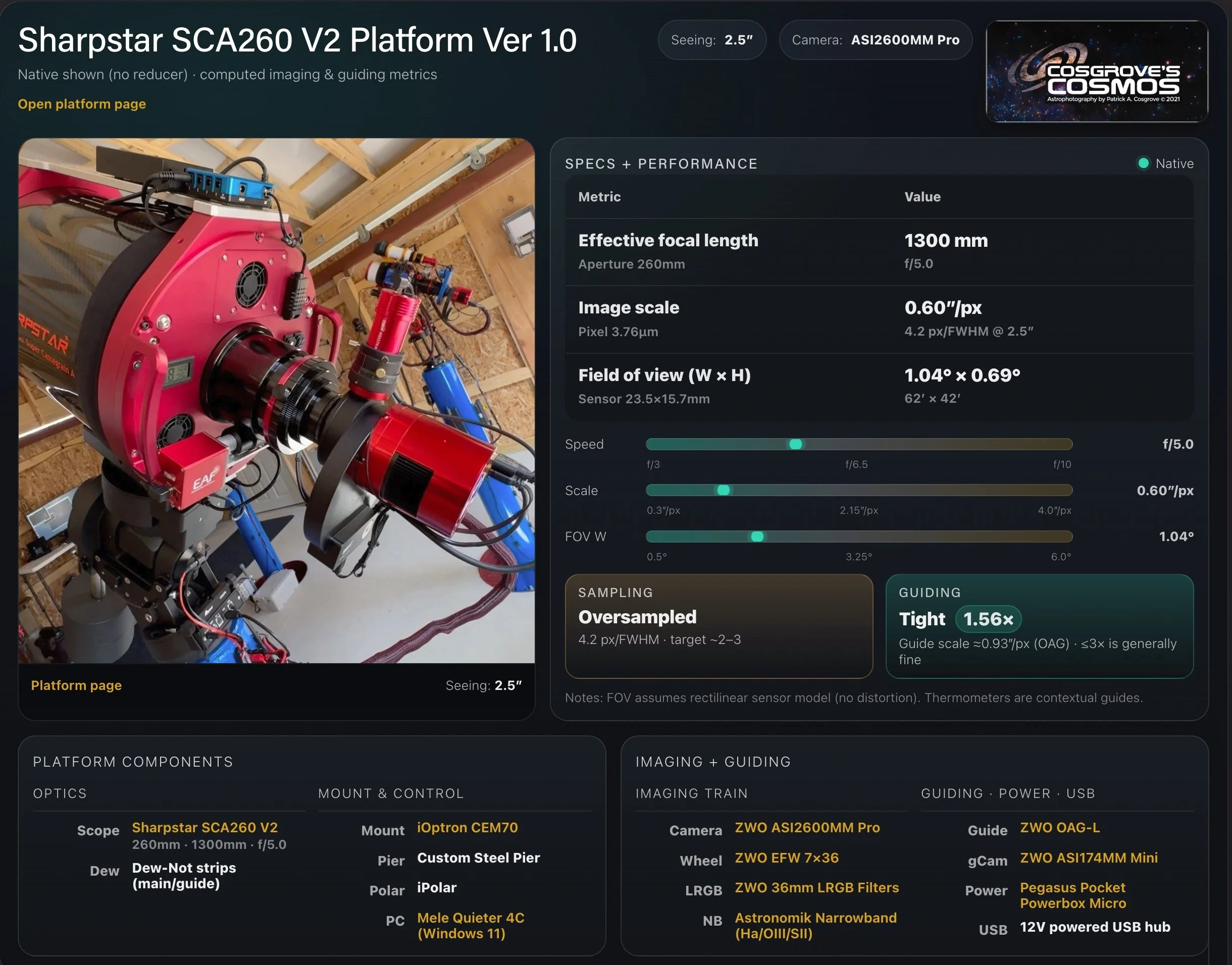
Platform used for this project
Software:
Capture Software: PHD2 Guider, NINA
Image Processing: Pixinsight, Photoshop - assisted by Coffee, extensive processing indecision and second-guessing, editor regret and much swearing…..
Image Processing Detail (Note: This is all mostly based on Pixinsight)
1. Assess all captures with Blink
Light images
Ha images:
Removed 2 -clouds
O3 images:
Removed 4 for clouds
S2 Images:
Removed 2 for clouds
Flat Frames
no issues seen on individual subs
Flat Darks
no issues seen
Darks
no issues seen.
Summary:
40 minutes lost to clouds
2. WBPP Script V 2.8.9
Load all files
Dark exp tolerance set to zero
Light exp tolerance set to zero
Pedestal auto for all frames
CC auto for all groups
Select max quality
Ref image set to auto
Selected the target folder
Drizzle 2x Square set
Executed in 33 minutes with no errors

WBPP setup.

Post Processing View of WBPP

WBPP Pipeline view
3. Import Master images and Rename

Master images. Ha, O3, S2
4. Create and Process the SHO Color Image
Create the Master_SHO image using the ChannelCombination Tool
This image is all green as expected. Normally, I would run DBE here, but this time I decided to try to get the color in the ballpark and then apply DBE to the color image. To do this, the first thing I did was run the NarrowbandNormalization script. See the panel before for the settings I ended up using.
Run NarrowbandNormalization. UPDATE: Do not run this yet. Run it after you go starless! This was a partial cause of my SXT issues.
This left a brown looking background and magenta stars, so I wanted to deal with that next,
First, the Magenta stars:
Invert the image - this makes the magenta stars green, so we can then run SCNR for green
Run SCNR for green at 95%
Invert the image gain
That fixed the stars, so now let’s fix the background
Run BackgroundNuetralization - see panel
That looks pretty good now.
Now let’s run DBE to remove the gradient and nonuniformities seen. This also adjusted the green balance.
Note: I think in the future I will continue to run DBE earlier on, as I normally do. I liked the color I had after NarrowbandNormalization and BackgroundNormalization, and the DBE shifted that.
Apply BXT on the color image with “Correct Only”
Run PFSImage: X = 11.97 Y=9.96. Not sure I believe this as the diffraction spikes might influence things.
Apply BXT with full correction. See panel-snap for values used. These were selected after interactive testing.
Run NXT = 0.75
Run STX to go starless. Preserve the stars

The initial SHO Image
After NarrowbandNormalization (click to enarge)

Narrowbandnormailization Params used.
Image Inverted. Magenta stars are now green. (click to enlarge)
SCNR 95% Green run (click to enlarge)

Image now inverted again - the stars look much better.
After BackgroundNeutrlalization. (click to enlarge)
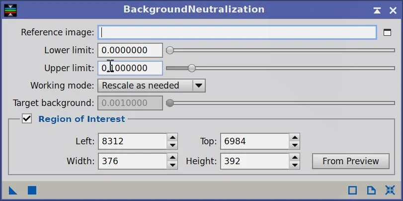
Params used.
DBE Sample pattern for SHO image. (click to enlarge)
SHO image before DBE. (click to enlarge)
SHO image after DBE. (click to enlarge)
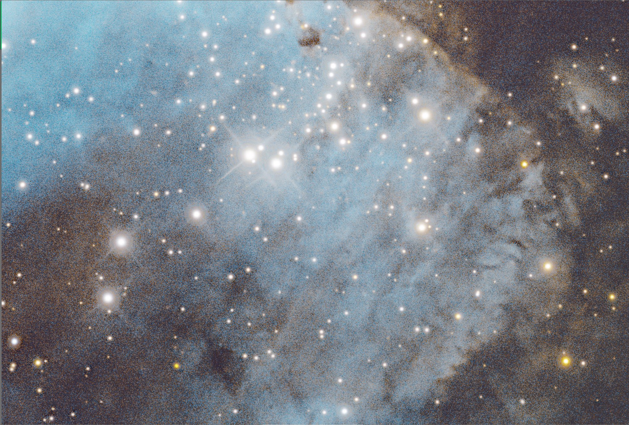
Background image subtracted. (click to enlarge)
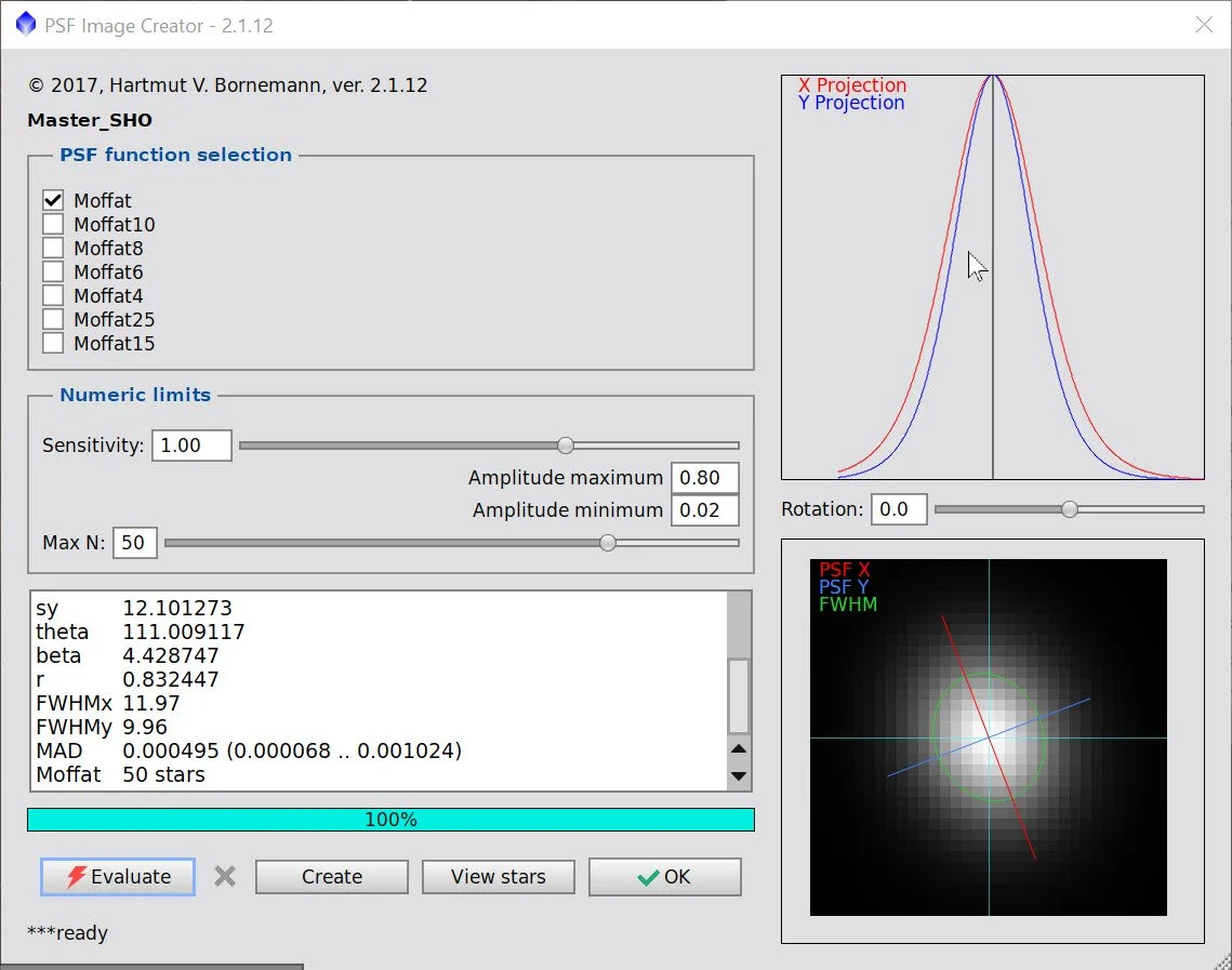
Star Sizes as determined by PFSIMage. Not sure it handles diffractions spikes correctly.
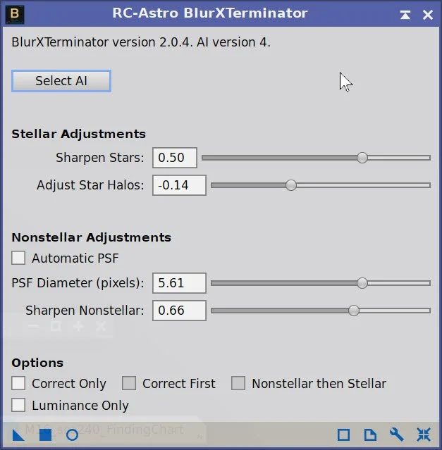
BXT settings used. Determined by trial.


SHO Image Before BXT, After BXT Crorrect Only, After BXT Full Correction, After NXT=0.75
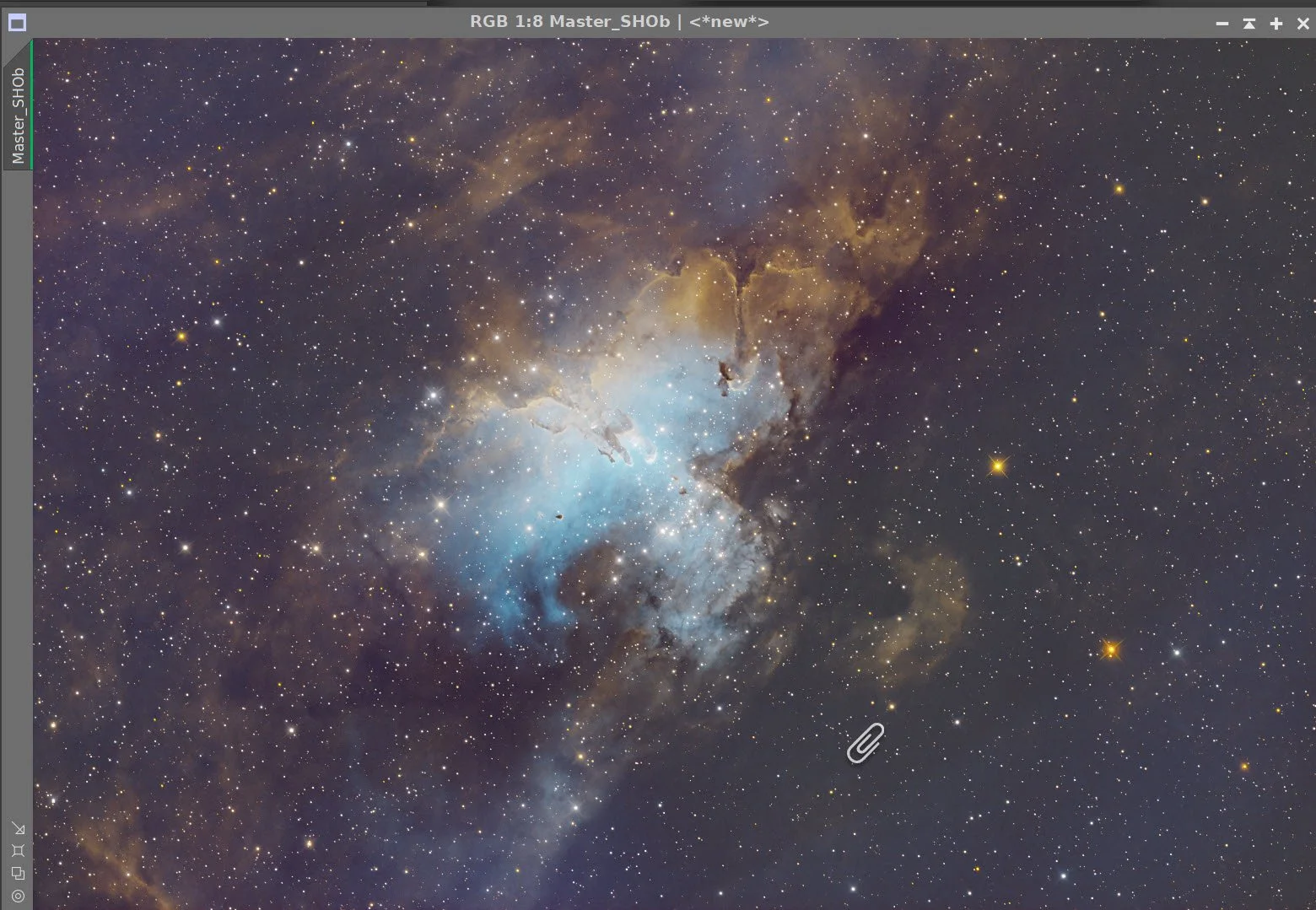
The Final Linear SHO image before star removal.
Master_SHO_Stars (click to enlarge)
Master_SHO_Starless (click to enlarge)
5. Process the nonlinear SHO Starless Image
Use the STF->HT method of going nonlinear
Use CT to adjust the overall tone scale and color
Use SelectRange to create a range mask that covers the lower exposure background of the image.
Apply the mask
Use CT to adjust the background to be darker and more neutral
Remove the mask
Run HDRMT with levels = 6 to open up the highlights a bit
Use CT to tweak the image
Use ColorSaturation to reduce purple tones and slightly boost blues.
At this point, I knew about the residual star blemishes, so I exported the starless image and fixed the blems with Photoshop’s healing brush .
Note: I should mention that this a fairly simplified processing that what I typically do. I usually get much more involved in color masks, sharpening, etc. Since this was a test, I simplified this. As a result, I did more active polishing on Photoshop than I normally do.
Initial SHO Starless Image (click to enlarge)
RangeMask targeting background (click to enlarge)
After HDRMT (click to enlarge)
After CT adjust (click to enlarge)
Use CT to adjust background. (click to enlarge)
CT adjust the entire image. (click to enlarge)


The final SHO Starless image after ColorSaturation Adjustment.
Example of residual star blemishes. (click to enlarge)
After Fixing in Photoshop click to enarge)
6. Process the SHO Stars-Only Image
Use the NarrowbandNormalization tool to fix up stat colors a bit
Take the linear star image and make it nonlinear by manually using the histogram tool.
Check over the image for any artifacts. Ring Artifacts were found on two bright yellow stars. These were not STX artifacts - these are due to the optics of the SCA260. I have heard other reports of this.
Export the star image to Photoshop and due to a crude correction before moving to the next step.
Starting SHO linear Star Image


After Adjustment with the NarrowbandNormalization tool.

Nonlinear Stars using Histogram tool
One of two ring artifacts found on bright orange stars (click to enlarge)
After a crude Fix n Photoshop (click to enlarge)
11. Add the Stars Back
Use the StarScreen script to add the stars back in.
The Final Starless Image. (click to enlarge)
The Final SHO Stars image. (click to enlarge)
The ScreenStars script combines the stars and starless images.

12. Move to Photoshop and do the final Polish
Export as 16-bit TIFF
Open in Photoshop
Rotate and Crop to create the final composition.
Use the Camera Raw filter to tweak color, tone, and Clarity.
Use Camera Raw ColorMix to adjust blue tones to darken them
Use the Lasso Tool to select the upper right corner and lighten it a bit
Use the Lasso Tool to select the lower right corner and lighten it a bit
Use the smart sector to grab the blue area
Apply a slight Gaussian blur filter to smooth it out a bit.
Do a final curve adjustment to make it snappier.
Add watermarks
Export various versions of the image
The final image sent to Photoshop for polishing (click to enlarge)

Lighten the lower right corner. (click to enlarge)
after a slight guassian blue of the blue area. (click to enlarge)

Lighten the upper right corner (click to enlarge)

Smart Select of the blue area (click to enlarge)
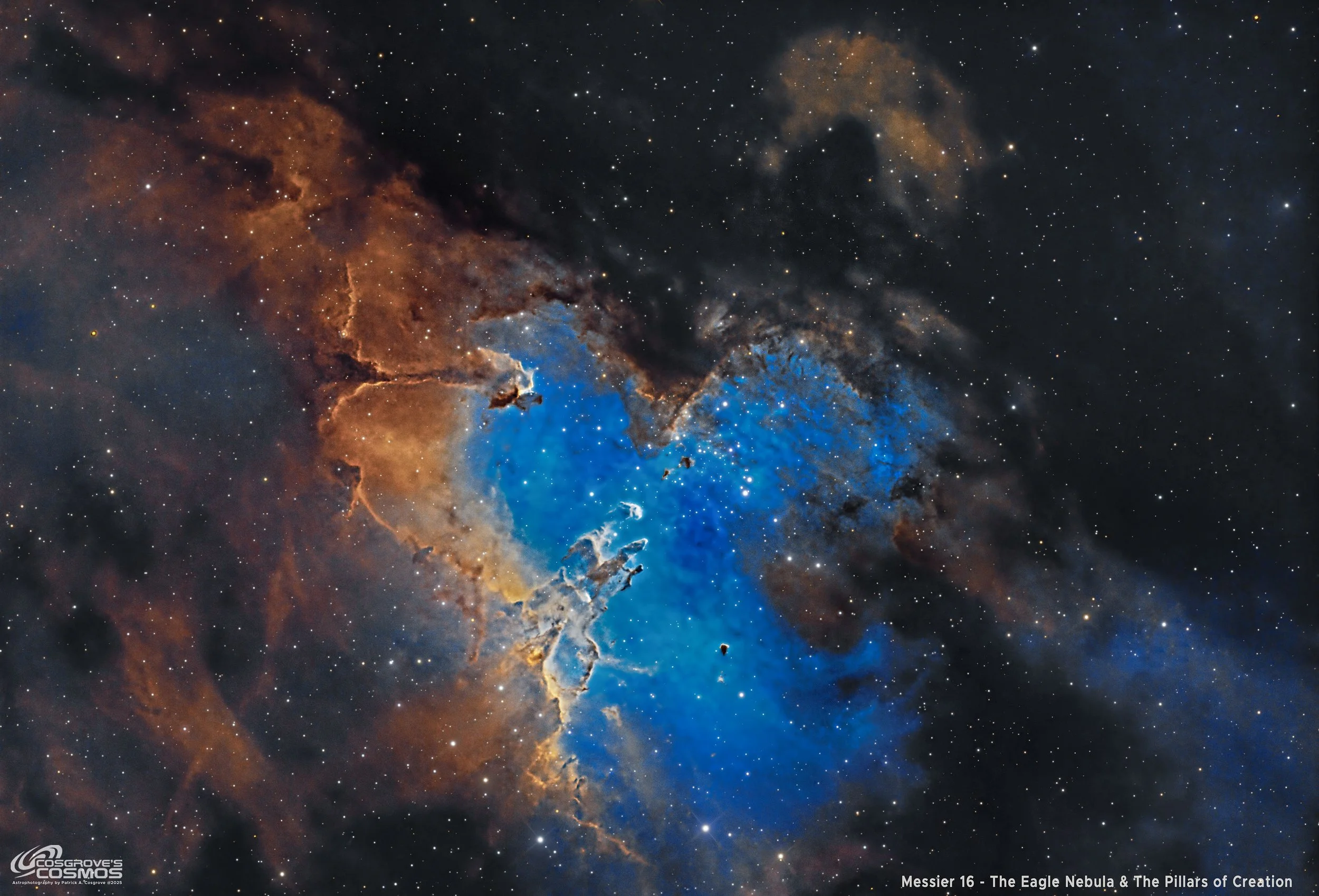
The Final Image after a CT curves adust to make it just a bit snappier.