
SH2-155 - The Cave Nebula 13.5 hours SHO (My 150th Project!)
Date: September 11, 2025
Cosgrove’s Cosmos Catalog ➤#0150

My Narrowband shot of the Cave Nebula! (click for access to full res image via Astrobin.com)
A dramatic SHO view of the Cave Nebula’s ionized rim and dust lanes; 13.5 hours captured with a 260 mm f/5 Cassegrain.
Table of Contents Show (Click on lines to navigate)
Background
My imaging rate saw a dramatic reduction over the past two years - a result of the move and all of the work that went into building my Whispering Skies Observatory. But now the observatory is up and running, and I am cranking out project after project. And that feels great!
This project is my 150th Imaging effort since starting my Astrophotographic journey!
My sincere thanks to those who have helped and supported me along the way! It is truly appreciated!
About the Target
Overview
The Cave Nebula is a broad, low-surface-brightness emission nebula (H II region) embedded in the Cepheus molecular-cloud complex.
In images, it shows a dark, cave-like hollow bounded by a bright, ionized rim. Surrounding this are reflection and dark nebulae mixed with lanes of dust.
Astronomically, Sh2-155 sits on the ionized edge of the Cepheus B cloud, where radiation from nearby massive stars sculpts the gas and dust and lights the rim. As a target, it’s expansive, subtle, and scientifically active — a classic northern object that rewards long integrations in narrowband or HaRGB.
Names and Designations
The object is most commonly listed as Sharpless 2-155 (Sh2-155). In amateur observing, it is also Caldwell 9 in Patrick Moore’s Caldwell catalogue, and in the Lynds Bright Nebulae, it appears as LBN 529. The popular name “Cave Nebula” became widespread through the Caldwell listing and the nebula’s appearance.
Historically, the nickname was sometimes applied to a different reflection nebula (vdB 152/Ced 201), but today, Sh2-155 is the usage most observers mean. For general background and nomenclature cross-checks, see NASA’s Hubble Caldwell 9 page and the Sh2-155 overview.
Location
Sh2-155 lies in the northern constellation Cepheus, near the Cepheus OB3 association. Modern sources place it at roughly 2,400 light-years (≈ 725 pc) from Earth. The cave-like rim marks the boundary where the ionizing radiation from OB stars meets the denser molecular material of Cepheus B.
History
The nebula entered the literature in 1959 when Stewart Sharpless published his second catalog of Galactic H II regions based on photographic surveys. Sh2-155 is the 155th entry in that list.
Decades later, Patrick Moore selected it for his Caldwell catalogue (as C9), which helped cement its common name and popularity with observers and imagers.
The Science
Sh2-155/Cepheus B is a textbook case of triggered star formation at an ionization front. X-ray (Chandra) and infrared (Spitzer) studies found a gradient in the ages of young stellar objects (YSOs) from the irradiated rim into the cloud interior — exactly what you expect if ultraviolet radiation from nearby massive stars is compressing the cloud and sequentially igniting star birth. One of the principal ionizing sources is the O-type star HD 217086 in the Cep OB3b subgroup; a nearby B-type star (HD 217061) illuminates associated reflection nebulosity. For accessible summaries and data, see Chandra’s press release “Trigger-Happy Star Formation,” along with detailed work on the structure of Cepheus B and its exciting stars.
Interesting Aspects and Observing Notes
Scientifically, the region is rich in embedded protostars, pillars, and dust globules at the interface between the H II region and the molecular cloud, making it a useful laboratory for testing feedback-driven star-formation models. Visually and in wide-field images, the Cave is part of a larger complex that rewards multi-filter approaches (Hα, [O III], [S II]) to bring out contrast between ionized gas and dust.
Annotated Image
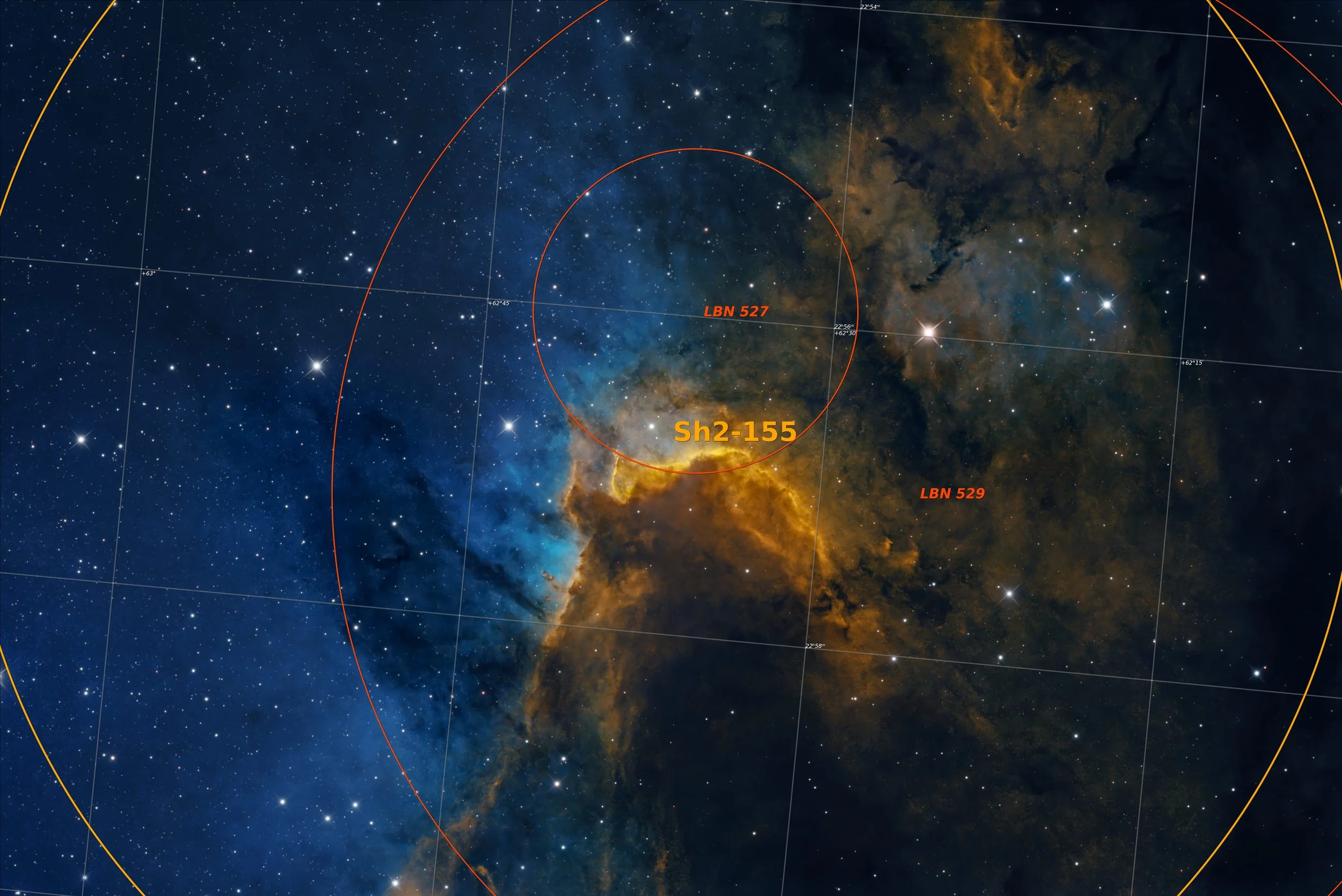
Image created with Pixinsight’s ImageSolver and AnnotateImage scripts.
Location in the Sky

Finder chart created with Pixinsight’s ImageSolver and FinderChart scripts.
About the Project
The last week in August was not at all bad weather-wise, and I took advantage of those nights that looked like they might be at least even partially clear.
I had scanned a few constellations for potential targets, and as I scanned, Cepheus, I saw the Cave Nebula. I was familiar with this as I had shot it once when I was very early in my astrophotography journey. This was an RGB version shot with an OSC, and I never had a chance to capture it in narrowband.
I thought this would be my opportunity.
When I assigned targets to scopes, I ended up making a somewhat surprising (to me) selection: the Sharpstar SCA260 for this project.
The other projects running concurrently ended up collecting data for 4 nights, but this project only had 3 nights of data collection. This was because I re-tasked the scope for one of those nights to shoot NGC 7331 and Supernova SN2025rbs before it faded from view!
Previous Efforts
This first imaging effort took place in November of 2020.
I was using my first scope, the William Optics 132 FLT, with my very first camera, the ASI294MC-Pro One-Shot-Color. This had approximately 3 hours of exposure. You can read about that Project HERE.
Below, you can see both images side by side:
Nov 2020, 3 hours with an OSC. (click to enlarge)
My current version - 13.5 hours in SHO (click to enlarge)
The new image offers a lot more detail, although it does have a much narrower field of view.
Data Capture
Data was collected on the nights of August 22, 24, and 31.
There is no rotator on the SCA260, so I kept the current rotation so I could reuse my flat calibration files.
The NINA sequence was set up to go after 300-second subframes at an aim cooler temperature of -10 degrees C.
On September 2nd, I captured new dark calibration files. I did this at night, as I seem to have a slight light leak in the configuration, and doing this at night guarantees there will be no problem.
After doing a blink, 18 total frames were removed due to clouds moving through the frame. This was a total loss of 1.5 hours from the integration.
Image Processing
Processing for this image, I followed my normal narrowband workflow, which looks like this:
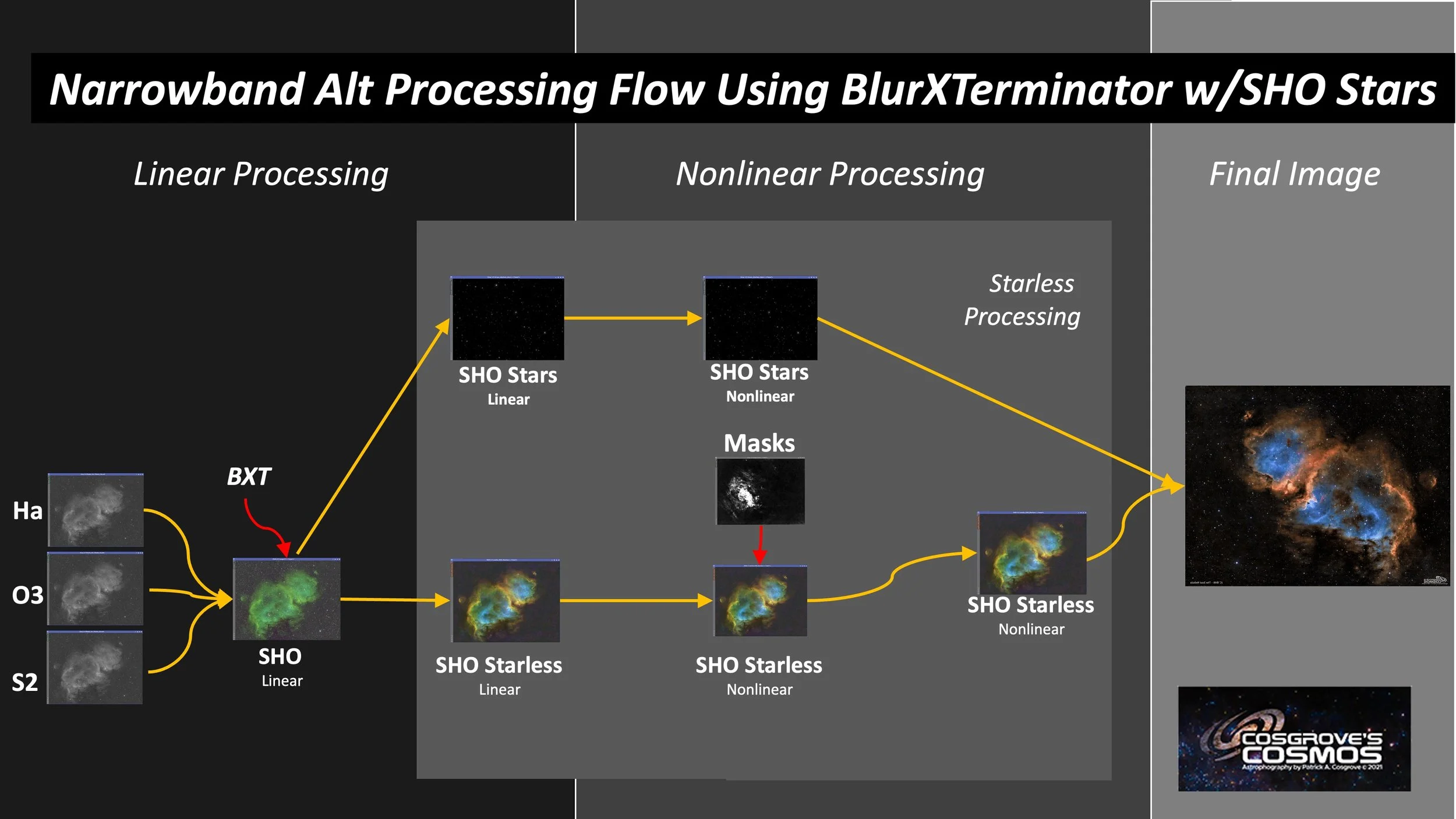
My SHO high-level workflow.
There were almost no surprises this time around.
The last time I did a narrowband nebula with this scope, I had problems with SXT removing stars and leading star blemish in the starless image. This caused a lot of artifacts to form. I also had issues with diffraction rings around the bright stars. So processing was a bear.
StarXterminator (SXT) has always worked exceptionally well for me, so this was a new experience. I consulted with Russ Croman, and he was kind enough to look at my data and see where things went wrong with SXT.
I had drizzle processed the image before doing BXT, NXT, and STX. This caused stars to be larger than what is used in SXT training.
I also ran NarrowbandNormaliser before BXT, NXT, and STX were applied. I did this because the guidance was to run SPCC on LRGB images before running these tools. If it helps to get the color right before doing this work, then that must also be true for narrowband - Right? Wrong! The low signal layers were stretched so much that the resulting noise pattern was different from what was seen in training.
So this time around: no drizzle processing, and I waited to do my NarrowbandNormalization adjustments until after I had run all of these tools.
SXT seemed to perform well, and I had negligible problems with residual star blemishes in the starless image! Yay!
I did see diffraction rings around the bright stars in the linear data. But by the time I had run, BXT, NXT, SXT, and had gone nonlinear, I really did not seem to be a problem! Double Yay!
My approach here is to create the color SHO image early, perform linear processes on this color image, and then proceed with nonlinear processes.
At that point, I always create two color masks:
a WarmMask - a color mask that includes all warm hues. With this mask, I do selective processing on the warm areas of the scene.
a CoolMask and do the processing I want on the cool hues of the scene.
I did that here. I found that most of the interesting details were found in the WarmLayer and used this to adjust not only color but also sharpness and contrast. The CoolMask was just used for Color and saturation adjustments.
Finally, this image had some interesting dark dust features. So, I created another mask using the Range Selection tool to isolate the dust and enhance it.
You can see the detailed processing walkthrough at the end of this post.
Results
The resulting image has a certain level of drama and mystery, which I appreciate. I am also pleased that the detail level was much greater than on my initial effort, and the color palette came out wonderfully.
The O3 signal was very weak and needed a lot of stretching to color this image. NXT did a good job, but there are some residual noise artifacts in the blue channel when you pixel-peep, so I could have done better with more integration.
More Info
🔭 Target Details
SIMBAD: Sh 2-155 (Cave Nebula) – Authoritative object record with coordinates, aliases (e.g., LBN 529, Caldwell 9), and links to the literature.
Aladin Lite Sky Atlas – Interactive sky viewer; search “Sh2-155” to explore DSS/IR overlays, field framing, and nearby objects.
Hubble Caldwell 9 (The Cave Nebula) – Overview page with context image showing the HST inset on the wider nebula, distance and observing notes.
NOIRLab Image: Sh2-155 (Cave Nebula) – KPNO Mayall 4-m wide-field image and caption describing the bright ionized rim on the edge of the Cepheus B cloud.
VizieR: Sharpless H II Regions (VII/20) – Catalog browser for the Sharpless list with parameters and original notes for entries, including Sh2-155.
📜 History & Naming
Sharpless (1959): A Catalogue of H II Regions (ADS) – Original paper that introduced Sh2-155, with methodology and photographic survey context.
Hubble — Caldwell Catalog Hub – Background on Patrick Moore’s Caldwell list that popularized common names like “Cave Nebula.”
Hubble Image Detail: Sh2-155 (WFPC2) – Official image page for the HST inset; credits and description of the region near the “cave” rim.
HEASARC: Sharpless H II Regions Database – NASA archive entry for the digitized Sharpless catalog with documentation and cross-references.
🔬 Science & Observations
Chandra Press: Trigger-Happy Star Formation in Cepheus B – Press summary of evidence that OB-star radiation compresses the cloud and triggers sequential star formation.
Chandra Photo Album: Cepheus B – Multiwavelength composite and discussion of YSO age gradients and disk fractions across the region.
Spitzer (Caltech/IPAC): Cepheus C and Cepheus B (IRAC) – Infrared view highlighting embedded structures and dust illuminated near Sh2-155.
JPL Photojournal: Cepheus C & Cepheus B Region – Two-instrument Spitzer composite with briefing notes and credits.
Getman et al. 2009 (ApJ): Disk Evolution in Cepheus B – Peer-reviewed study detailing the YSO population, age gradient, and triggered star-formation scenario.
💡 Interesting Facts & Outreacg
APOD: SH2-155 — The Cave Nebula (2014-11-06) – Narrowband composite emphasizing H-alpha/[O III]/[S II] structure with a clear “cave” silhouette.
APOD: SH2-155 — The Cave Nebula (2017-03-23) – Wide-field view with color mapping and a concise explanation of distance and location in Cepheus.
APOD: The Cave Nebula in Infrared from Spitzer (2019-06-11) – IR perspective revealing pillars and embedded activity not obvious in visible light.
NOIRLab Zoomable: Sh2-155 – Pan/zoom interface to inspect faint dust lanes and plan mosaics or framing.
AstroBin: Sh2-155 Image Gallery – Curated community images (varied FOVs and palettes) useful for composition ideas and filter choices.
Capture Details
Lights
Data was captured on the nights of August 22, 24, and 31, 2025
The number of frames is after bad or questionable frames were culled.
53 x 300 seconds, bin 1x1 @ -10C, gain 100, Astronomik 36mm diameter 6nm Ha Filter
55 x 300 seconds, bin 1x1 @ -10C, gain, 100, Astronomik 36mm diameter 6nm O3 Filter
55 x 300 seconds, bin 1x1 @ -10C, gain 100, Astronomik 36mm diameter 6nm S2 Filter
Total of 13 hours 30 minutes
Cal Frames
30 Darks at 300 seconds, bin 1x1, -10C, gain 100
30 Dark Flats at each Flat exposure times, bin 1x1, -10C, gain 100
15 Ha Flats
15 O3 Flats
15 S2 Flats
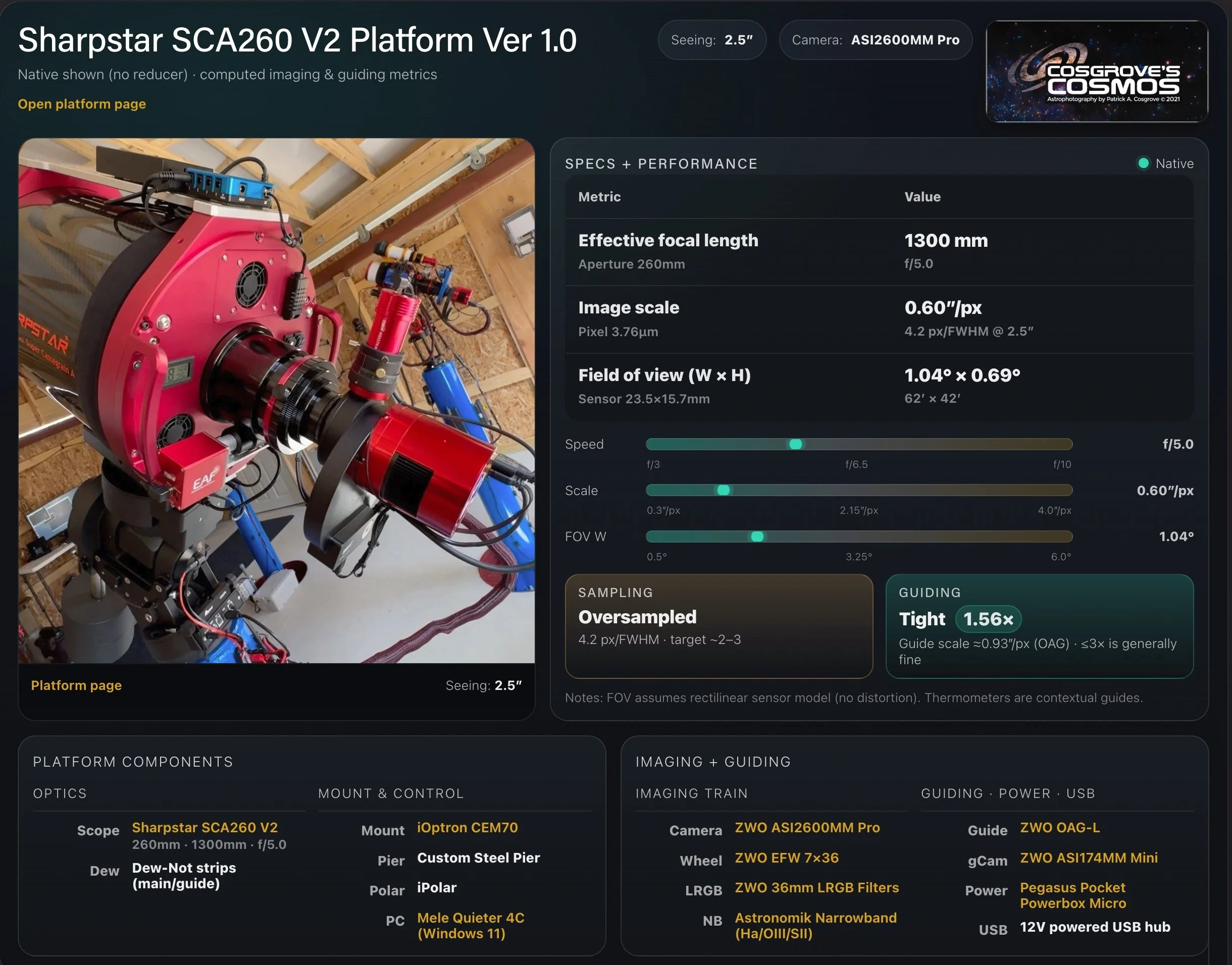
Platform used for this project
Software:
Capture Software: PHD2 Guider, NINA
Image Processing: Pixinsight, Photoshop - assisted by Coffee, extensive processing indecision and second-guessing, editor regret and much swearing…..
Image Processing Detail (Note: This is all mostly based on Pixinsight)
1. Assess all captures with Blink
Light images
Ha images:
Removed 11 -clouds
O3 images:
Removed 3 for clouds
S2 Images:
Removed 4 for clouds
Flat Frames
No issues seen on individual subs
Flat Darks
No issues seen
Darks
No issues seen.
Summary:
1.5 hours minutes lost to clouds
2. WBPP Script V 2.8.9
Load all files
Dark exp tolerance set to zero
Light exp tolerance set to zero
Pedestal auto for all frames
CC auto for all groups
Select max quality
Ref image set to auto
Selected the target folder
Executed in 33 minutes with no errors
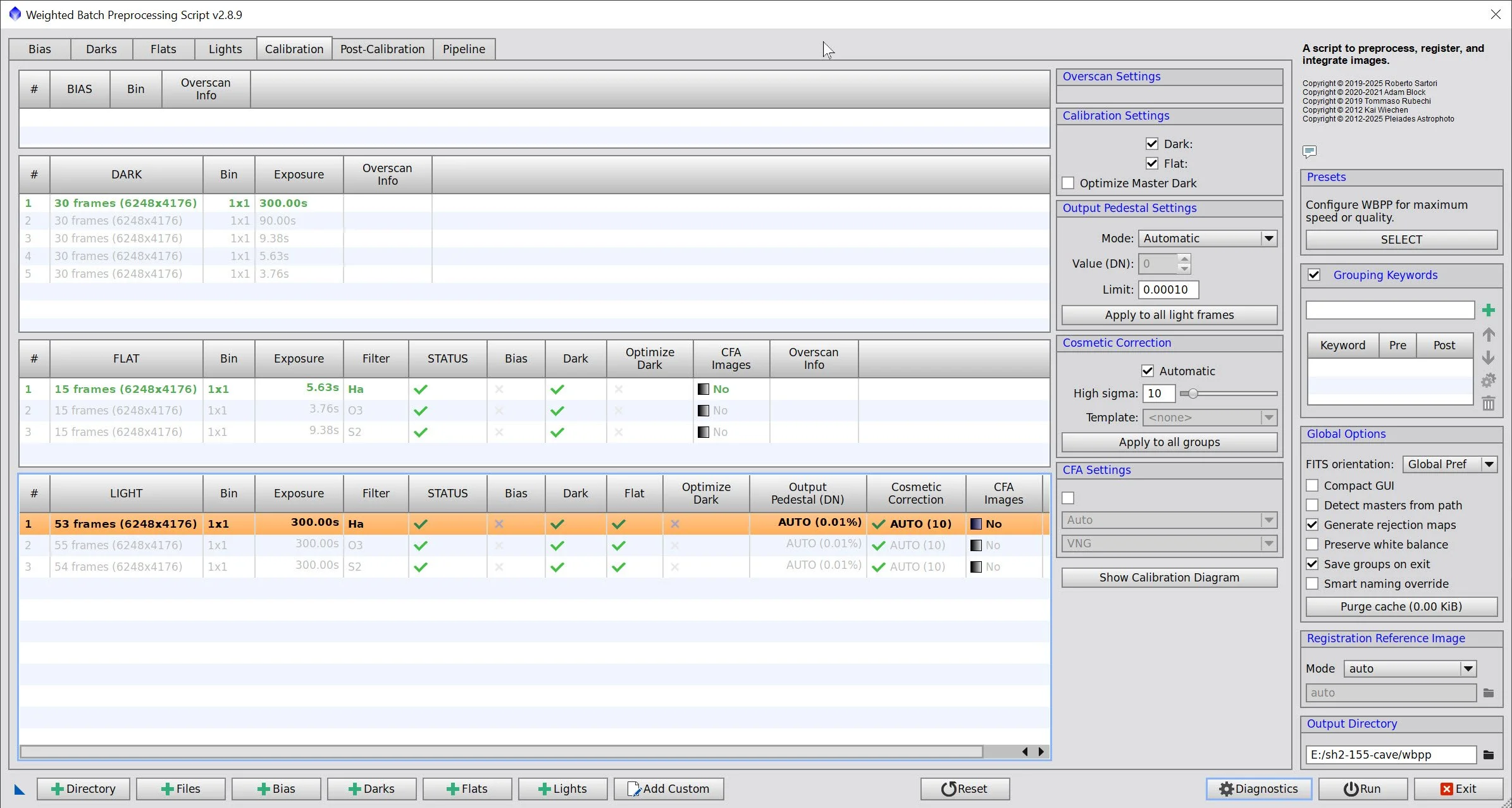
WBPP setup.

Post Processing View of WBPP
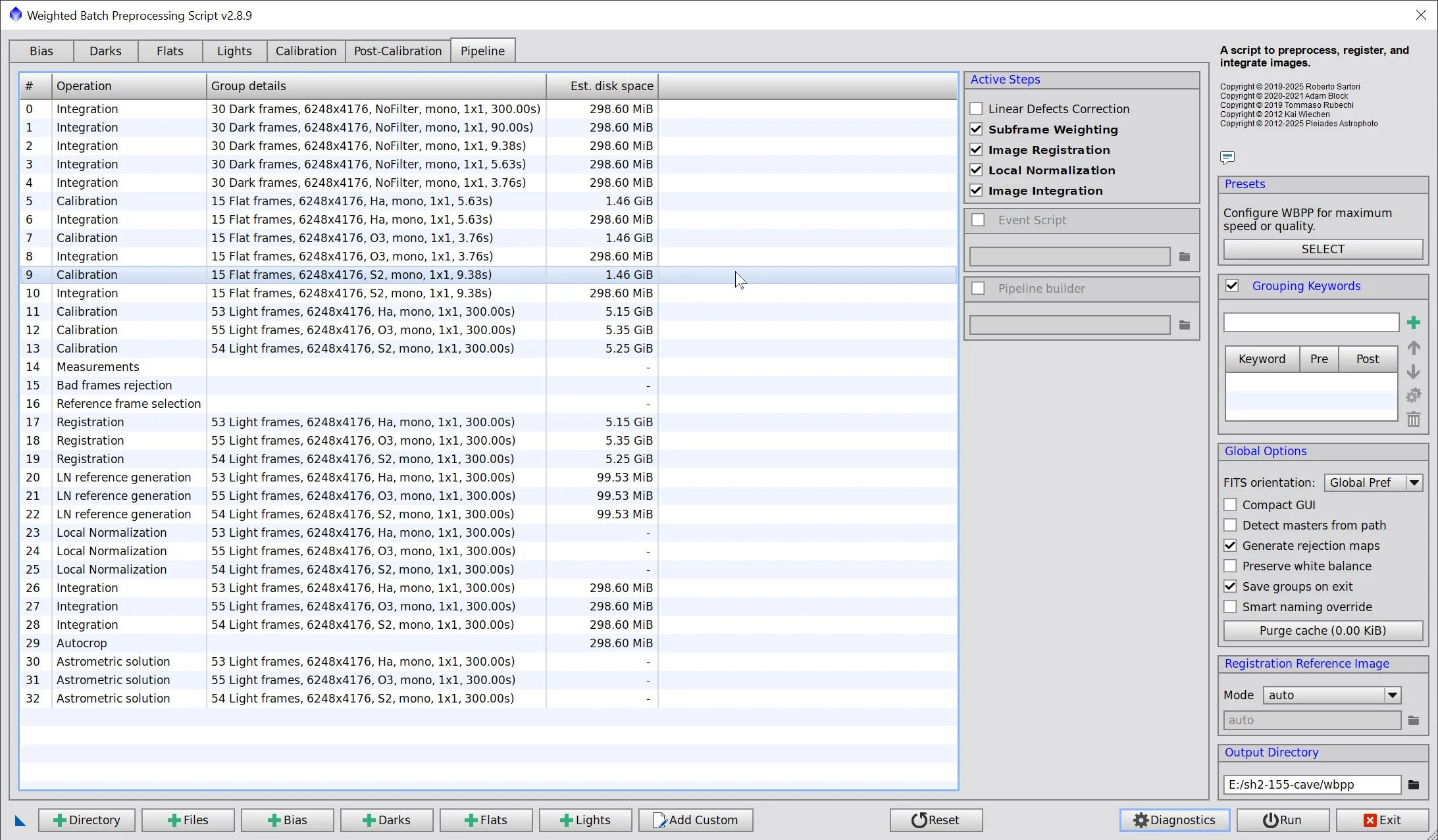
WBPP Pipeline view
3. Import Master images and Rename
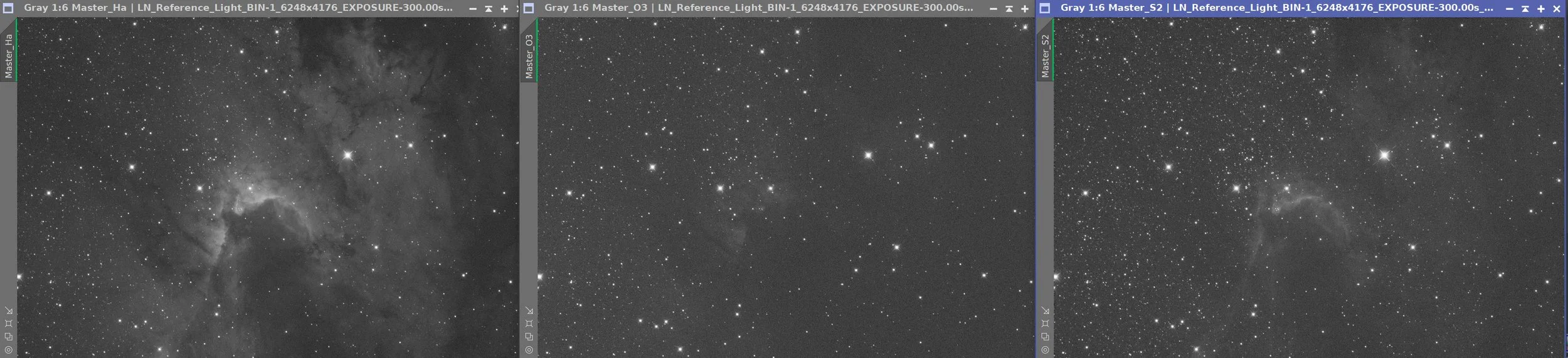
Master images. Ha, O3, S2
4. Create and Process the SHO Color Image
Create the Master_SHO image using the ChannelCombination Tool.
I did not see much evidence of a gradient, so I opted not to do a DBE run.
Apply BXT on the color image with “Correct Only” (This corrects for any stars that are not round - not a lot gets done here, really)
Run PFSImage: X = 2.11, Y = 2.22. I'm not sure, but I believe these are the diffraction spikes that might be influencing things.
Apply BXT with full correction. See panel-snap for values used. These were selected after interactive testing. ( I find I get the best nonstellar results when the correction is about 1/3 larger than the measured star sizes)
Run NXT V3 - See panel snapshot below.
Run STX to go starless. Preserve the stars
Run NarrowbandNormalization script with params shown in the screensnap below (this starts to clean up the narrowband stars)
Get rid of the Magenta tones
Invert (turns magenta into green so I can use SCNR to remove it)
Run SCNR for Green at 0.90
Invert

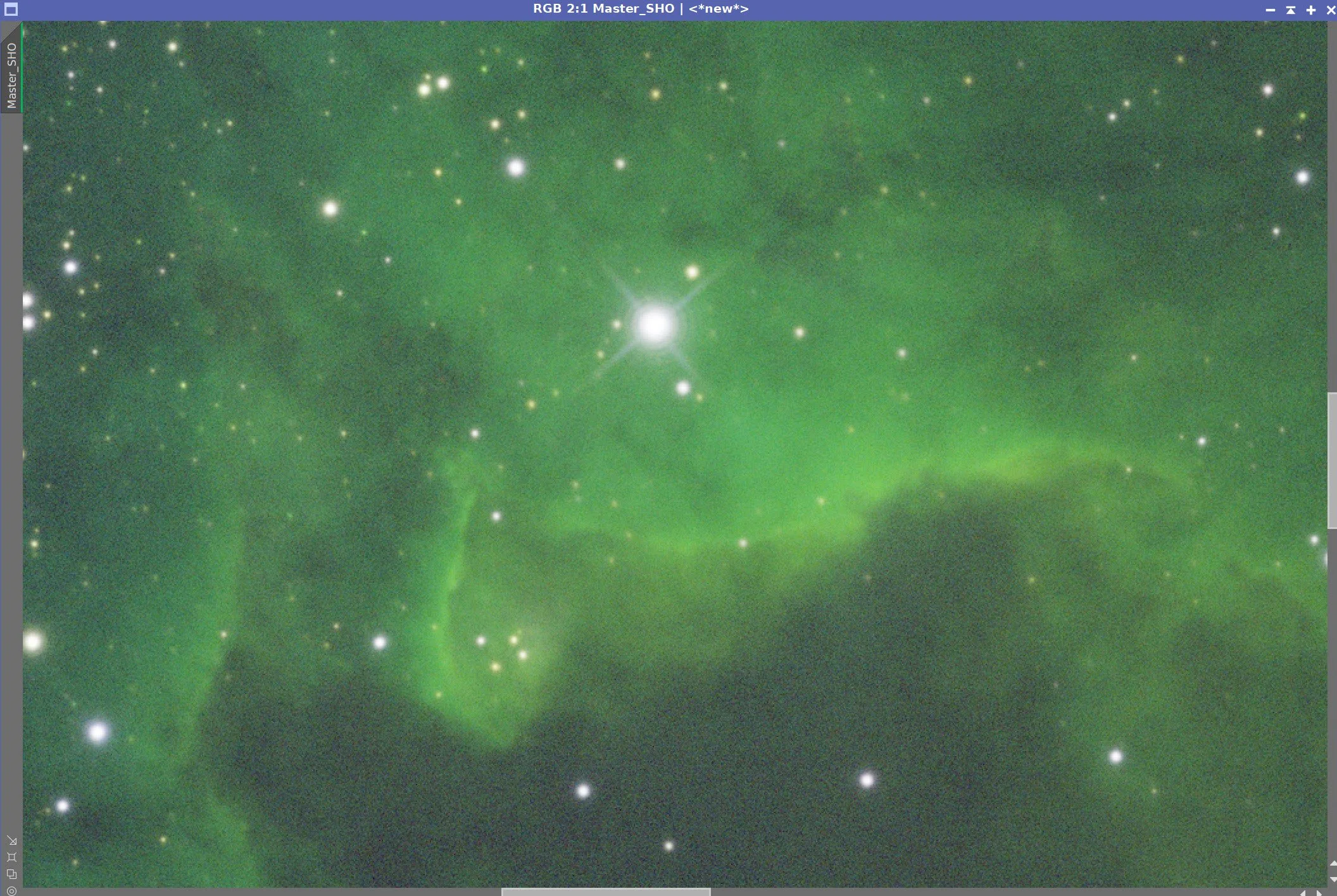
The initial SHO Image
Star Sizes as measured. (click to enlarge)
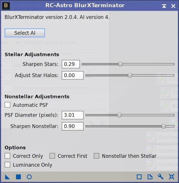
BXT Params used.
NXT Params used (click to enlarge)
SCNR 95% Green run (click to enlarge)
Params used.


SHO Image Before BXT, After BXT Correct Only, After BXT Full Correction, After NXTV3
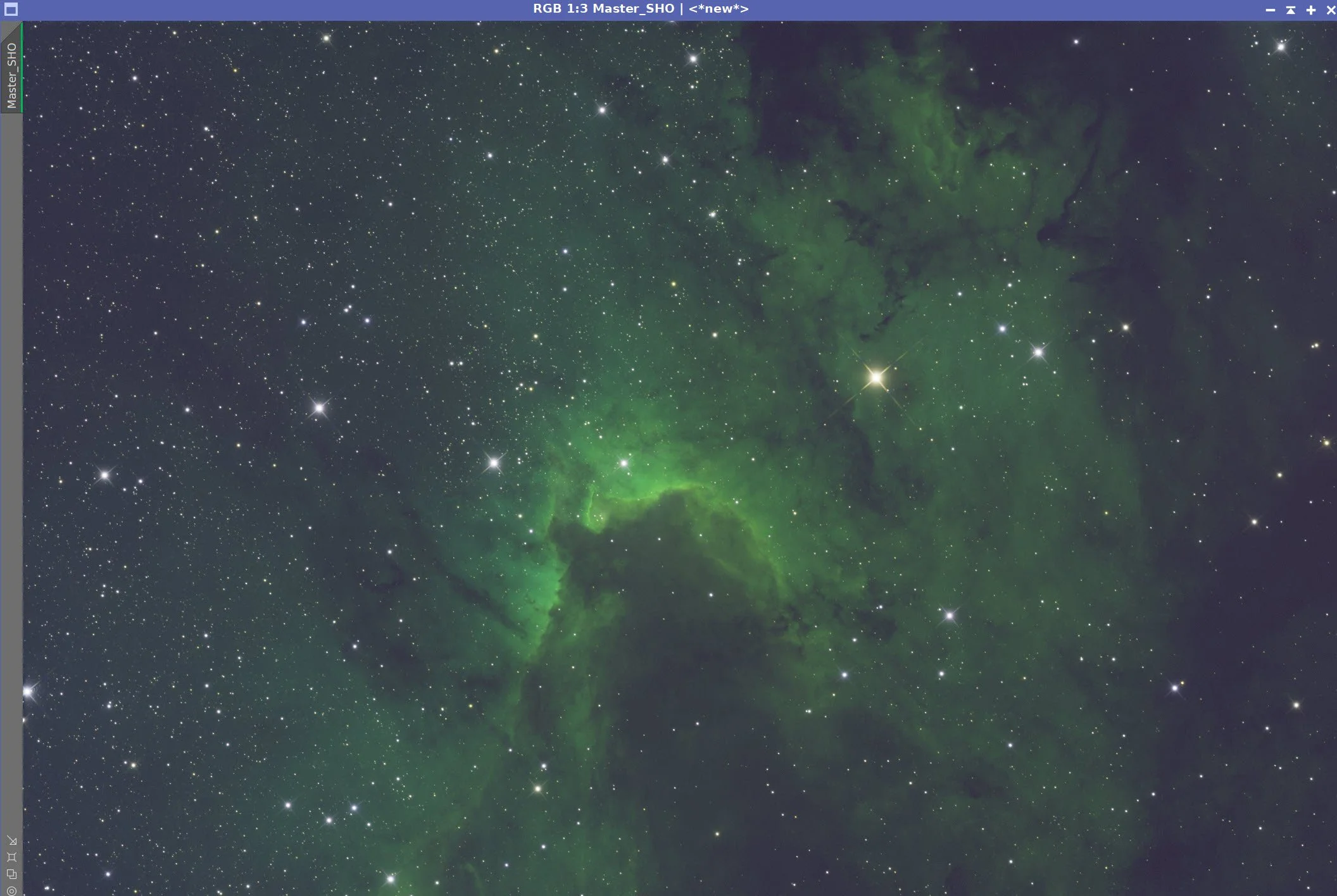
The Final Linear SHO image before star removal.
Master_SHO_Stars (click to enlarge)
Params used for NarrowNormalization
Master_SHO_Starless (click to enlarge)
After NBNormalization (click to enlarge)
SCNR for Green at 0.9 (click to enlarge)
Invert to get to the final Master SHO Starless image (click to enlarge)
5. Process the nonlinear SHO Starless Image
Use the STF->HT method of going nonlinear.
Apply CT and adjust. (initial chance to shape the tone and color position)
Create the WarmMask with the ColourMask Process with a hue range of 330 to 65 and a mask blur of 2.0.
Apply the WarmMask:
CT to set color and saturation
LHE1 to enhance small-scale detail. Radius 46, Max Contrast 2.0, Amount 0.5, 8-bit Histogram
LHE2 to enhance small-scale detail. Radius 300, Max Contrast 2.0, Amount 0.35, 10-bit Histogram
Create the CoolMask with ColourMask Process with a hue range of 169 to 259 and a mask blur of 2.0.
Apply CoolMask and do a CT for tonescale, color, and saturation.
Remove the mask, apply NXT with the params shown in the screensnap below
(There is a lot of interesting dark dust. So let’s try to enhance that with the next few steps. )
Using RangeSelection, create a DarkMask with a range of 0.14 to 0.18 with a smoothing of 5
Apply the mask
Do a CT adjust
Apply LHE to enhance small-scale features: Radius: 50, Max Contrast 2.0, amount 0.35, 8-bit histogram.
Apply MLT Sharpening. See ScreenSnap for params used.
Remove Mask and do another round of NXT - see screensnap for params used.
Create two final images with CT - A lighter one, and a darker one
Initial SHO Starless Image (click to enlarge)
Creating the WarmMask. (click to enlarge)
Apply CT with WarmMask (click to enlarge)
LHE2 applied with WarmMask (click to enlarge)
CoolMask (click to enlarge)
After CT adjust (click to enlarge)
WarmMask (click to enlarge)
LHE1 applied with WarmMask (click to enlarge)
Creating the CoolMask
CT with CoolMask (click to enalrge)
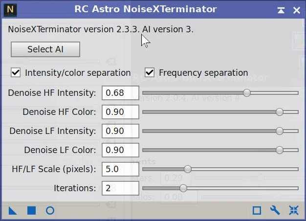
NXT Params used.
NXT Applied (click to enlarge)
The DarkMask (click to enlarge)
Apply LHE for small-scale with DarkMask (click to enlarge)
MLT Sharpening with DarkMask applied (click to enlarge)
CT with DarkMask applied (click to enlarge
Sharpening Params used (click to enlarge)

NXT Params used for the next operation
Another round of NXT (click to enlarge)
FInal Version - Lighter (click to enlarge)
Final Version Darker (click to enlarge)
6. Process the SHO Stars-Only Image
Adjust stars a bit in the linear state using the NarrowbandNormalization script - see the screensnap for the parameters used.
Use the STF->HT method of going nonlinear.
Use Seti Astro NB->RGB stars
Extract R, G, B layers as this tool wants mono files as input (Why? I have no idea - it’s rather inconvenient to my workflows) Use the NarrowbandNormalization tool to fix up star colors a bit.
Master Stars image. (click to enlarge)
After NBNormalization (click to enlarge)
Params used in NBNormalization (click to enlarge)
Seti Astro NB-toRGB-Stars Script
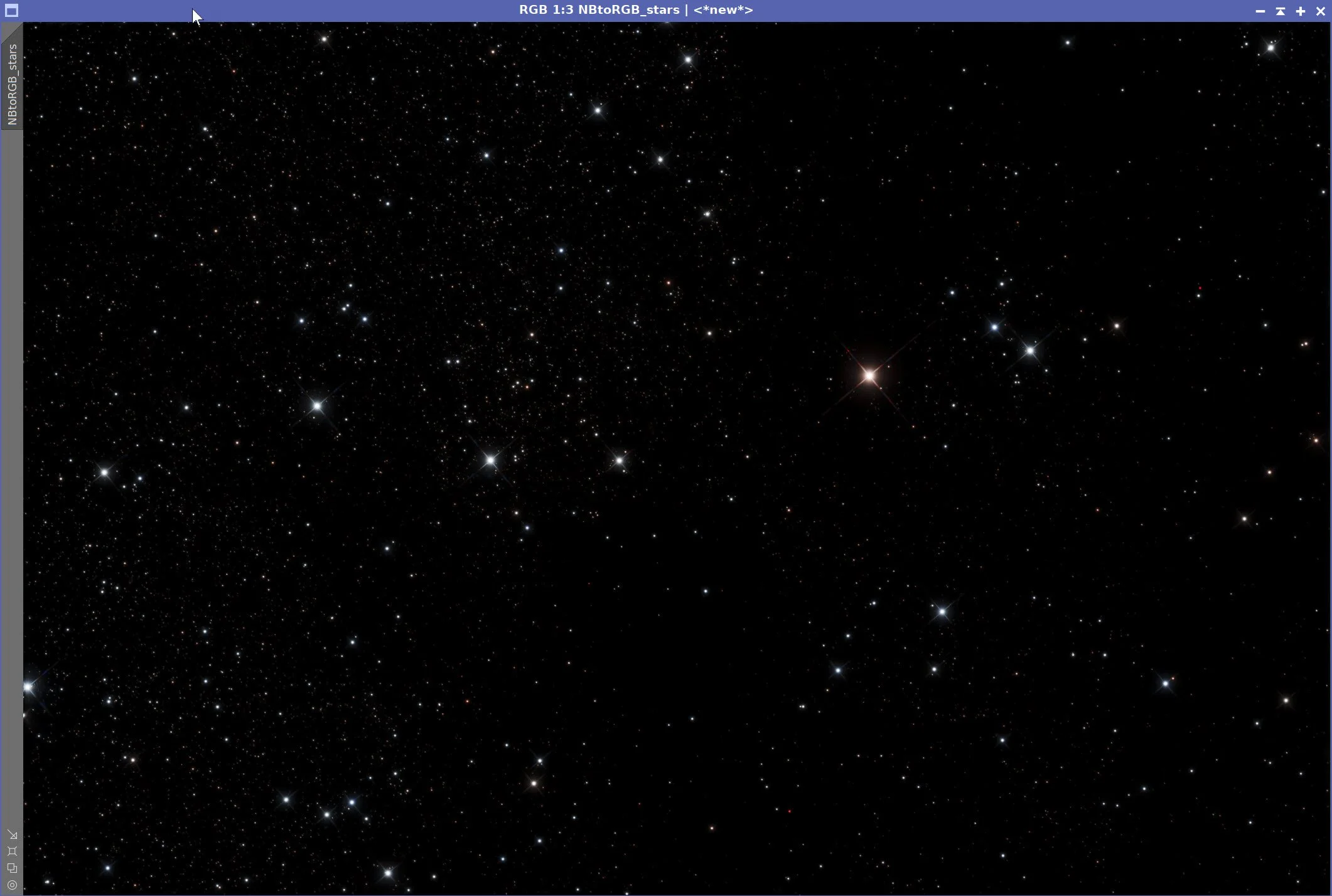
Final Stars
11. Add the Stars Back
Use the StarScreen script to add the stars back in using both lighter and darker versions of the Starless image
I liked both!
After asking for feedback from friends, I decided move the light version into Photoshop, and darken the right side of the image and keep the lightness of the left side!
The ScreenStars script combines the stars and starless images.
With Light Starless (Click to enlarge)
With Dark Starless (Click ot enlarge)
12. Move to Photoshop and do the final Polish
Export as 16-bit TIFF
Open in Photoshop
Crop slightly to move the right edge in a bit
Use the Camera Raw filter to tweak color, tone, and Clarity.
Use Camera Raw ColorMix to adjust blue tones to darken them
Use the Lasso Tool to select the right half of the image and darken
Add watermarks
Export various versions of the image

The final version!(click to enlarge)