
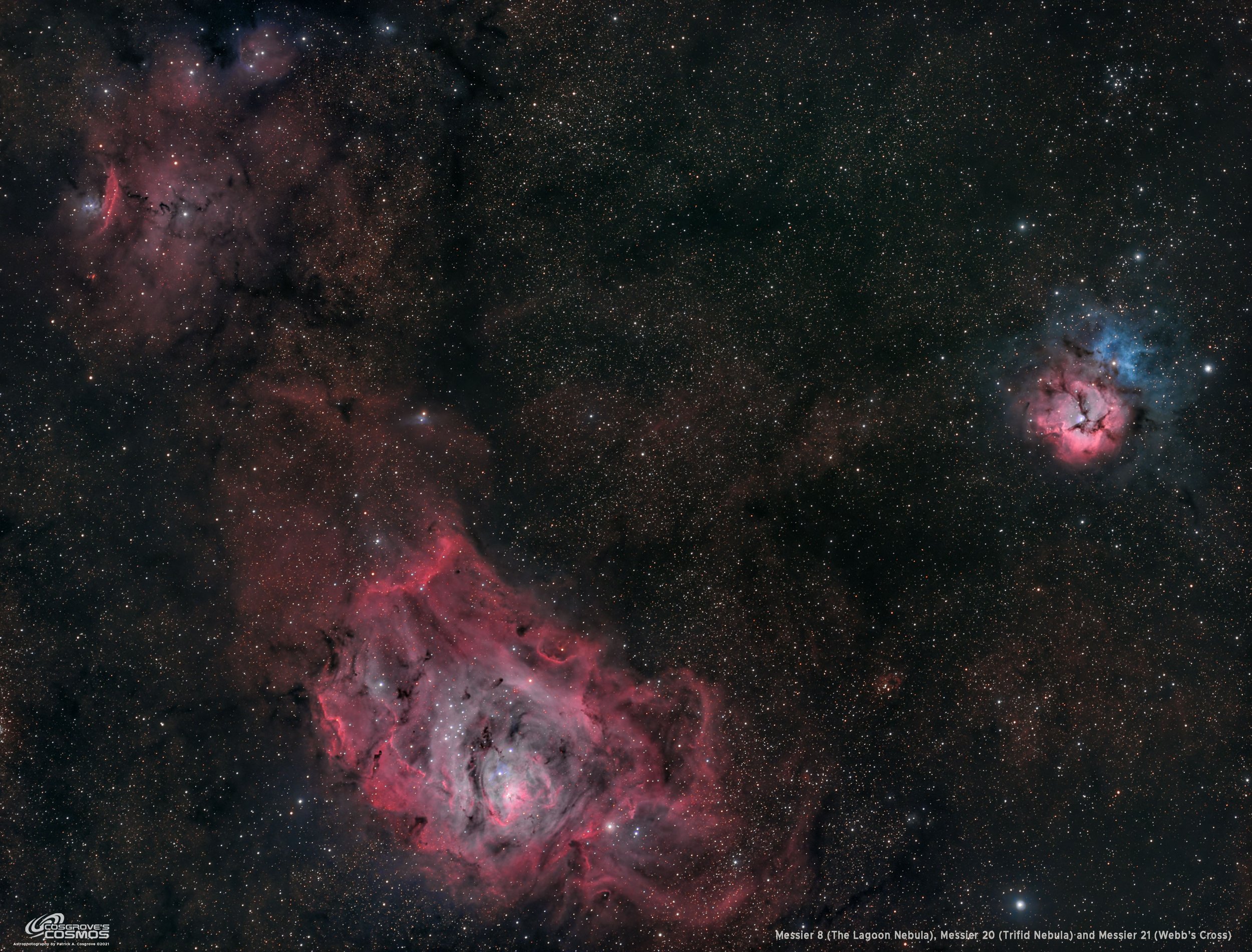
Messier 8, 20, and 21: A Rich Region in Sagittarius - 3.9 hours in HaRGB
Date: Aug 18, 2022
Cosgrove’s Cosmos Catalog ➤#0109

A widefield shot of a very rich region that includes the Lagoon nebula (M8), The Trifid Nebula (M20), Webb’s Cross (M21). (click image for a full resolution view voa Astrobin.com)
Table of Contents Show (Click on lines to navigate)
About the Target
For most imaging projects I do, the goal is a portrait of one object or target.
But sometimes, it is interesting to take a group shot.
And just like any group shot, you can struggle with getting everyone into the frame and deciding on which poses work best.
In today’s shot, we have the broader field coverage of the Askar FRA400 scope coupled with a ZWO ASI1600MM-Pro camera - which covers about 2.5 x 2 degrees.
I focused on a rich area in the constellation Sagittarius, which includes Messier 8, Messier 20, and Messier 21. In addition, we have a less known nebula whose shape reminds me of an animal’s paw or perhaps an arm ending in a fist! This area seems to be covered by a series of catalog entries that include IC 4585, NGC 6559, IC 1273, IC 1274, and several others that can be seen in the annotated version of the image below.
Messier 8 - The Lagoon Nebula
M8 Is a huge cloud of molecular gas and dark dust located about 4000-6000 light-years away in the constellation of Sagittarius. This is a large emission nebula that is bright enough to be seen with the naked eye. Within the cloud is the open cluster NGC 6530, and a bright central feature is known as the Hour Glass.
Messier 20 - the Trifid Nebula
M20 is known by the common name “The Trifid Nebula” and by NGC 6514. It is a star-forming region in the constellation of Sagittarius and is located about 4100 light-years away. Here is what Wikipedia has to say:
It was discovered by Charles Messier on June 5, 1764. Its name means 'three-lobe'. The object is an unusual combination of an open cluster of stars, an emission nebula (a relatively dense, red-yellow portion), a reflection nebula (the mainly NNE blue portion), and a dark nebula (the apparent 'gaps' in the former that cause the trifurcated appearance also designated Barnard 85). Viewed through a small telescope, the Trifid Nebula is a bright and peculiar object and is thus a perennial favorite of amateur astronomers.
Messier 21 - Webb’s Cross
M21 is an open cluster located 3,930 light-years away in the northeast section of Sagittarius. It was discovered by Charles Messier in 1764.
While there are a few bright blue stars in the grouping, most of the stars are tightly packed and are fairly dim. This cluster has a magnitude of 6.5, which means it cannot be seen with the naked eye and needs at least binoculars to see. This cluster has about 50-100 stars that are all very similar in age, suggesting that their formation was triggered by a comment event.
IC 4685 Region
This is a great example of a nebula that has red emission, blue reflection, and some dark dust components. This nebula is located very close to M8 - the Lagoon Nebula. It is most likely an extension of that nebula. As can be seen in the annotated version of the image, they are many other destinations associated with this region.
The Annotated Image
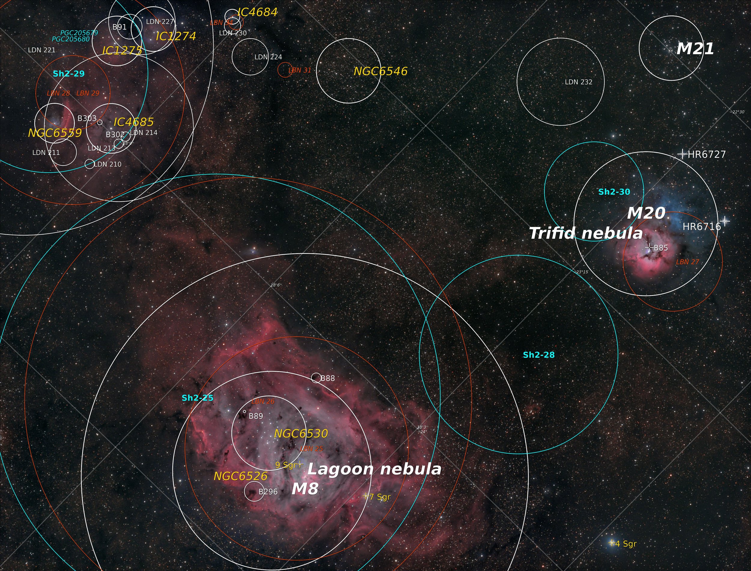
This annotated image was created in Pixinsight, using the ImageSolver and Annotate Image Scripts.
The Location in the Sky

This finger chart was created in Pixinsight using the FinderChart process.
About the Project
Introduction
A few minutes of introduction for this project by yours truly… Now featuring my new Annomated Logo intro and Outro!

Choosing the Target
We recently had a wonderful sequence of five clear, moonless nights! As I prepared for imaging during this cycle, I had already picked out targets for my Astro-Physics 130mm platform and my William Optics 132mm platform. I needed to find a target that would do well with my widefield Askar FRA400 platform.
One of the things I do when trying to find targets is to find out what constellations are rising above my eastern tree line about when it starts to get dark out. In this case, Sagittarius was well positioned. I then went to Astrobin.com and searched for astrophotos that were taken in that constellation - hoping to find some inspiration. I saw one image that had M8 and M20 in the same field. It was a pleasing image, and it started me thinking about the idea of a group shot rather than a single subject.
The Sagitarrius region of the sky is looking inward - towards the center of the galaxy - rather than away from it. Because of this, the Milky Way is the dominant factor here, and many objects are packed into a relatively small area of the sky. With my FRA400, I have the widest field I can cover among the scopes I now use. I wondered how many interesting objects I could fit within its frame.
To that end, I ran Sequence Generator Pro and pulled up the Framing and Mosaic Wizard.
I searched for the M8 region and explored several possible image compositions that I thought might be interesting. In the end, I chose the framing you see in the final image. This would let me highlight M8 and M20 - and would also cover the open cluster M21 and the region that has an interesting “fist”-like formation that I was not very familiar with. I liked the idea of combining the well know objects with those that are less known.
Data Capture
I decided to use 120-second subs and capture data using the Ha, R, G, & B filters. My thinking was to use the Ha data in place of the traditional Luminance channel.
I programmed my subs and got ready for the first night of shooting. The good news is that this region cleared my trees shortly after astronomical twilight ended. So I ensured I had the FRA400 platform ready to go when this region was clear.
The other issue I had to deal with is that this was low in my southern sky. The east and west tree lines are closest together here, which meant my time on target was limited. I could probably get about 2 hours a night or a little less. Given this, the chances for deep integration were very limited.
Things seemed to run OK, and because my automation was working pretty well, I did not watch what was going on very carefully. I paid a price for this lack of diligence!
At some point during the second night, I noticed that my tracking errors were much larger than I would normally tolerate. This raised a red flag. This sometimes happens when a cable is dragging or snagging. So I investigated this and determined that was not the case. I looked at the PHD2 data more carefully and noticed that the errors were concentrated in the Declination axis. Hmmm.
The CEM26 has a lot of backlash in the Dec Axis. This is just something I deal with. This is caused by having too low a tension in the drive belt for that axis. IOptron provided me with a procedure to adjust this. It’s not hard to adjust - but the problem seems to be that the slack is taken up by moving a block holding the gear - pulling it tight- and then tightening down on a screw to hold it there. The housing is plastic, and the screw, even when tight, seems to allow it to slip over time. So some level of backlash is always a problem. But by going through PHD2’s excellent documentation, I have configured the Dec tracking algorithm to deal with this intelligently, and I have always had good results with this setup.
So I looked at the PHD2 guiding parameters. Surprisingly, a check box allowing backlash compensation was no longer set! This is a big deal as I need backlash compensation for this mount! I have never changed it, and I don’t know how this parameter was ever modified. I re-selected this and then watched the subsequent guiding. All looked good again!
I looked back at my captured subs, and many of them had either elongated stars or trails! Sigh…. Looks like I would be losing some data due to this issue!
After this correction, the results were again reasonable and stayed that way for the remainder of the capture period.
Data Analysis
Blink analysis showed that the data looked pretty good in general. If I zoomed into a tighter preview, I could see that some had elongated star issues, so a total of 14 subs were culled at this point. There goes almost a half-an-hour of subs!
Sample of tracking errors seen. (click to enlarge)
Sample of tracking errors seen. (click to enlarge)
Sample of tracking errors seen. (click to enlarge)
After running WBPP, which calibrated and aligned the data, I ran Subframe Selector.
I use this to screen the subs for FWHM (star bloat) and Eccentricity (elongated stars). Removing the outlying frames with these issues has really helped improve the quality of my master images. I expected in this case that I would be seeing more subs that needed to be removed.
A total of 6 more frames were removed. This was not as bad as I expected. After WBPP, I had 4 hours and 4 minutes of data. After running SubframeSelector, I removed another 12 minutes of data for a new total of 3 hours and 52 minutes of data. Given that the FRA400 is an f/5.5 system, about 4 hours of data should not be too bad. More is ALWAYS better, but sometimes you get what you get!
Previous Attempts
While I have never taken this particular field and framing before, I have previously captured images of M8 and M20.
Messier 8:
My first image ever, from August of 2019, can be seen HERE.
My second attempt at M8 in June of 2020 can be seen HERE.
My third attempt was in August of 2021, which can be seen HERE.
Messier 20:
Here are those images for your viewing convenience:
M8 - Aug 2019 - first image ever! (click to enlarge)
M8 in RGB, June 2020 (click to enlarge)
M8 in Narrowband SHO, taken in Aug of 2021 (click to enlarge)
M20 in RGB, taken in June of 2020. click to enlarge)
M20 - my first Mono image ever! Taken in July 2020. (click to enlarge)
Image Processing
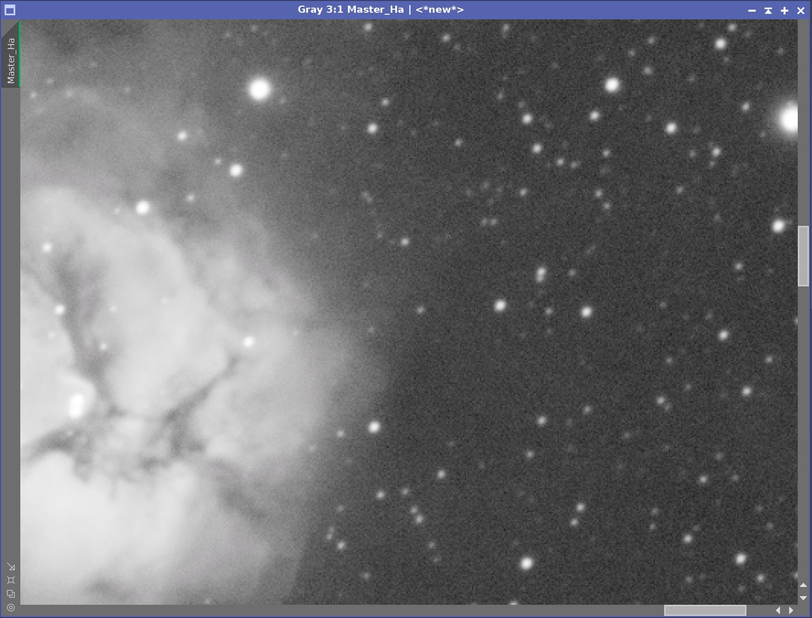
I originally intended to use the Ha channel as the Luminance in an LRGB processing treatment. This changed when I saw the Ha Master Image. There is so much Ha signal in the region that the Ha nebulae looked thick and almost featureless. This was born out when I tried doing a Ha image insertion into the RGB image with LRGBCombination. The resulting image shows the bright portions of the nebulae to be more opaque, with a loss of detail. On the other hand, the fainter portions of the nebulae show better, and the stars are not as dominant.
So I decided to create a synthetic luminance using the ImageIntegration process to combine the information from the Ha, R, G, and B data.
I then did a fairly standard process flow for LRGB, using LRGBCombnation to insert the synthetic lum image. In this case, the brighter portions of the nebula have more details, but the stars clearly dominate the image, and the fainter portions of the nebulae are also not seen as well.
Based on this, I thought the best approach was to use a blend of Ha and Lum in the final image.
The Ha Master Image. Note how opaque it seems around M8 and M20. (click to enlarge)
The RGB image after Ha Insertion. Note the opaque nature of the bright nebulae (click to enlarge)
The Synthetic Luminance image - I felt this would work better. (click to enlarge)
The RGB image after Lum insertion. In this version the nebulae has more detail but faint portions are less evident and the stars clearly are dominating the scene. (click to enlarge)
Even with the blend of Ha and Lum influences, the sheer number of stars dominates the image.
To deal with this, I plan to use Bill Blanshan’s excellent PixleMath equations to dial the stars back to a manageable level.
Discussion of Results
In general, I was pretty pleased with my group shot. Each comes across as well-defined, and there is plenty of eye candy in the scene that makes it interesting.
While I need up losing almost an hour of subs between the subframes that were removed during the Blink and the SubFrameSelector processes - again - removing such questionable frames is the right thing to do.
A detailed Processing Walk-Through is provided for this image at the end of the posting…
More Information
Wikipedia: Messier 8
Nasa.gov: Messier 8
Wikipedia: Messier 20
Nasa.gov: Messier 20
Wikipedia: Messier 21
Meesier-objects.com: Messier 21
Wikisky.org: IC 4685
Capture Details
Lights Frames
Data was collected over five nights: July 28,-July 31, and Aug 2.
Number of subs after Blink and SubFrameSelector analysis and removal
10 x 300 seconds, bin 1x1 @ -15C, Gain Zero, Astronomiks 6nm Ha
37 X 120 seconds, bin 1x1, @ -15C, Gain Zero, ZWO Red
35 X 120 seconds, bin 1x1, @ -15C, Gain Zero, ZWO Green
19 X 120 seconds, bin 1x1, @ -15C, Gain Zero, ZWO Blue
Total of 3 hours 52 minutes
Cal Frames
25 Darks at 300 seconds, bin 1x1, -15C, gain Zero
12 Flats at bin 1x1, -15C, gain Zero - for Ha, R,G,B filters
25 Dark Flats at Flat exposure times, bin 1x1, -15C, gain unity
Software
Capture Software: PHD2 Guider, Sequence Generator Pro controller
Image Processing: Pixinsight, Photoshop - assisted by Coffee, extensive processing indecision and second-guessing, editor regret, and much swearing…..
Capture Hardware:
Scope: Askar FRA400 f/5. 6 Astrograph
Focus Motor: ZWO EAF 5V
Guide Scope: William Optics 50mm guide scope
Guide Scope Rings: Wiliam Optics 50mm slide-base Clamping
Ring Set
Mount: IOptron CEM 26
Tripod: Ioptron 1.5” Tripod
Camera: ZWO ASI1600MM-Pro
Filter Wheel: ZWO EFW 1.2 5x8
Filters: ZWO 1.25” LRGB Gen II, Astronomiks 6mm Ha, OIII,SII
Guide Camera: ZWO ASI290MM-Mini
Dew Strips: Dew-Not Heater strips for Main and Guide
Scopes
Power Dist: Pegasus Astro Powerbox Advanced
USB Dist: Pegasus Astro Powerbox Advanced
Polar Alignment Cam Iplolar
Software:
Capture Software: PHD2 Guider, Sequence Generator Pro controller
Image Processing: Pixinsight, Photoshop - assisted by Coffee, extensive processing indecision and second-guessing, editor regret and much swearing…..
Click below to see the Telescope Platform version used for this image
Image Processing Walk-Through
(All Processing done in Pixinsight - with some final touches done in Photoshop)
1. Blink Screening Process
Ha
One frame was removed for trees
Some frames show slight star elongation - but I have so few I will have to do the best I can by using rejection to clean these up.
Red
Some trails
Some frames with elongations - 4 frames removed
Green
Removed 5 for elongation
Minimal gradients
Some trails
Blue
Some trails
Six frames were removed for trees
Flats
Collected for the first three nights. Data looks good
Dark flats
Collected for the first night - data looks good
Darks
Get Darks from the 7-26-22 cal files.
2. WBPP 2.4.5
Reset everything
Load all lights
Load all flats
Load all darks - Darks 120 and 300 from fpa400 7-29-22
Add the “Night” keyword
Select - maximum quality
Reg reference - auto - the default
Select output directory
Enable CC for all light frames
Pedastal value - auto for Ha frames
Darks -set exposure tolerance to 0
Deselect integration mode - just cal and alignment
Map flats and darks across nights
Ran with no problems

WBPP Calibration view.

Post Calibration View.
3.0 Use SubFrameSelector to analyze the Calibrated subs
After WBPP ran, I used SubFrameSelector to check the quality of my subs.
Subs for each filter were loaded into the tool, and metrics were computed. FWHM and Eccentricity were the key metrics I used in this analysis. Screenshots for each filter are attached below.
Ha images: 0 deleted for having too high an FWHM or Eccentricity value
R images: 1 deleted for having too high an FWHM or Eccentricity value
G images: 2 deleted for having too high an FWHM or Eccentricity value
B images: 3 deleted for having too high an FWHM or Eccentricity value
I was not very aggressive in what I eliminated for the Ha as I had relatively few subs here.
Ha Sub FWHM - Note eliminated frames (click to enlarge)
Red Sub FWHM - Note eliminated frames (click to enlarge)
Green Sub FWHM - Note eliminated frames (click to enlarge)
Blue Sub FWHM - Note eliminated frames (click to enlarge)
Ha Sub Eccentricity - Note eliminated frames. (click to enlarge)
Red Sub Eccentricity - Note eliminated frames (click to enlarge)
Green Sub Eccentricity - Note eliminated frames (click to enlarge)
Blue Sub Eccentricity - Note eliminated frames (click to enlarge)
4. Integration
ImageIntegration
ImageIntegration was run for each Master image.
The same setup was used for each run.
ESD was chosen for rejection.
Large scale rejection checked - 2x2
A sample panel for ImageIntegration can be seen below

ImageIntegration panel settings.
Rejection High - Ha (click to enlarge)

Rejection High - Green: (click to enlarge)
Rejection High - Red: Note trails removed (click to enlarge)
Rejection High - Blue: (click to enlarge)
5. Crop all of the images
A common crop level was selected, and DynamicCrop was used to trim all of the master frames.
The edges were remarkably clean. Only a little had to be removed from the left-most edge.
6. Dynamic Background Extraction
DBE was run for each image using the subtraction method. Below are the Sampling plans, the before image, the after image, and the removed background images.
Because of the extensive nebulosity, mostly outer edge sampling was done.
DBE: Ha Sampling (Click to enlarge)
Ha image Before DBE (click to enlarge)
Ha image After DBE (click to enlarge)
Ha background removed (click to enlarge)
DBE: Red Image Sampling (Click to enlarge)
Red Image Before DBE (click to enlarge)
Red Image After DBE (click to enlarge)
Red background removed (click to enlarge)
DBE: Green Sampling (Click to enlarge)
Green image Before DBE (click to enlarge)
Green Image After DBE (click to enlarge)
Green background removed (click to enlarge)
DBE: Blue Sampling (Click to enlarge)
Blue image Before DBE (click to enlarge)
Blue Image After DBE (click to enlarge)
Blue background removed (click to enlarge)
7. Create and Process the Linear Color Images
Create an initial RGB image by running ChannelCombination
Run PCC
Running Noise XTerminator with a value of 0.5 in linear mode

Initial Master_RGB

PCC Regression Line

Master_RGB after PCC.
Before and After application of RC Noise XTerminator with a value of 0.5
8. Process the Linear Ha Image
Prep for deconvolution
Run PFSImage and create the PFS
Run StarMask to create the initial LDSI image. (see StarMask settings below in the panel screenshot)
Use HT (see panel screenshot below for curve uses) to boost the LDSI mask.
Select multiple Previews of the Ha image for Decon parameter exploration.
Iteratively tested deconvolution with various parameters until the best result is obtained.
Run Deconvolution on the Ha image
Run Noise XTerminator in linear mode with a value of 0.5

PFSImage Panel after PSF has been computed for Ha

Ha PFS

StarMask settings used to create the LDSI mask.

HT boost settings for the LDSI mask

The final LDSI image for Ha

Preview areas selected for Deconvolution parameter testing.

Final Decon Values used for Ha


Linear Ha Image Before and After Decon, and After Noise XTerminator 0.5
9. Create a Synthetic Luminance Image and complete its Linear Processing
Write out master Ha, Red, Green, and Bue images as files (needed for the next integration step)
Run ImageIntegration
load the master files just written out
Default integration method
No rejection methods
Run - creating the Master L file
Prep for Deconvolution
Create a PFS-Lum image by running PFSImage Script
Create LDSI image
Run the Starmask process with parameters seen in the screen snap below
Run HT to boost the resulting star mask using the HT curve seen in the snap below
Select a few image previews for testing deconvolution parameters
Run Deconvolution using the PFS image and the LDSI Image - iteratively test parameters until the best result is obtained.
see final parameters below.
Run Noise XTerminator with a value of 0.5

ImageIntegration set up for creating synthetic Lum

The relative weights applied by ImageIntegration to the four input files to create the Synthetic Lum image. Note how strong the Red and Green contributions are!

PSFImage Panel for the Lum image.

The Lum PSF image

StarMask setting used to create original LDSI map

HT transform to boost LDSI map

The final Lum LDSI image.

The three preview regions set up to explore decon settings for the Lum image

The final settings on the Decon Panel for the Lum image.
Lum Image Before and After Deconvolution, and After Noise XTerminator 0.5
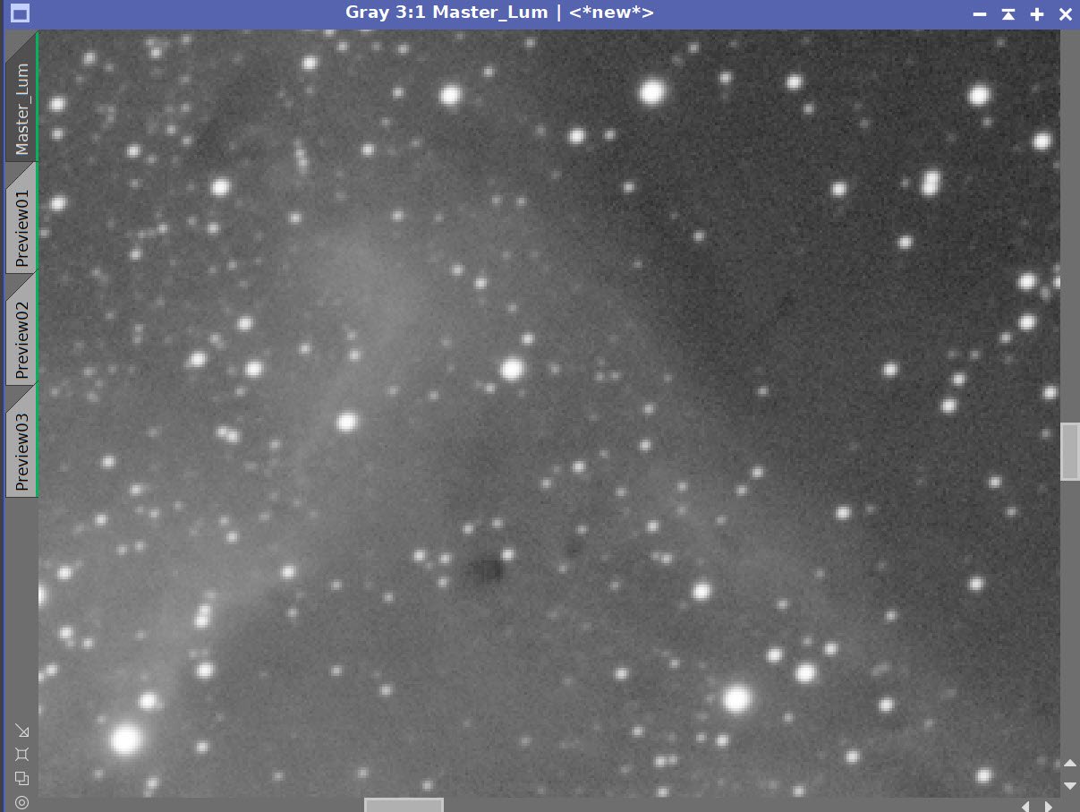
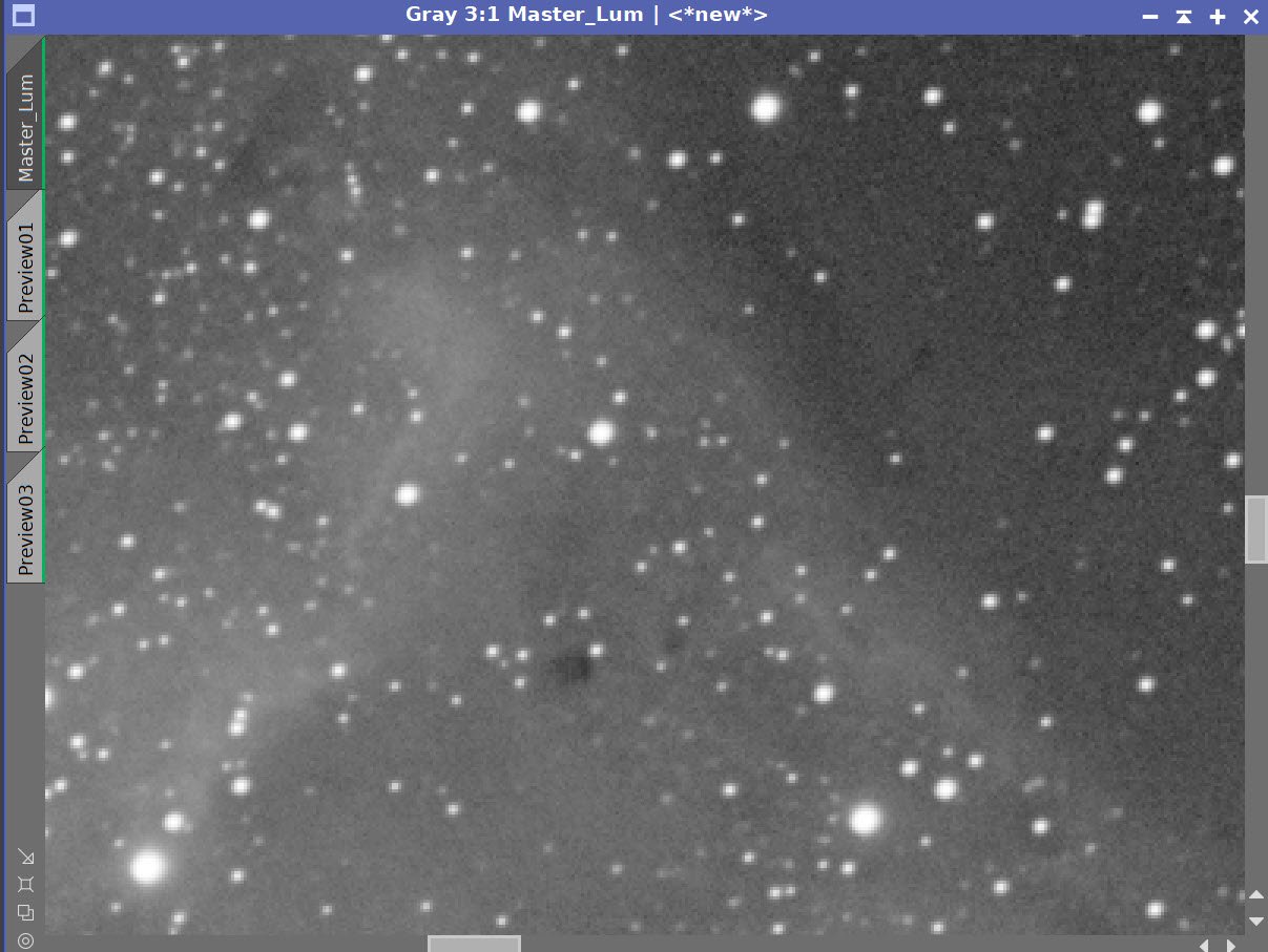
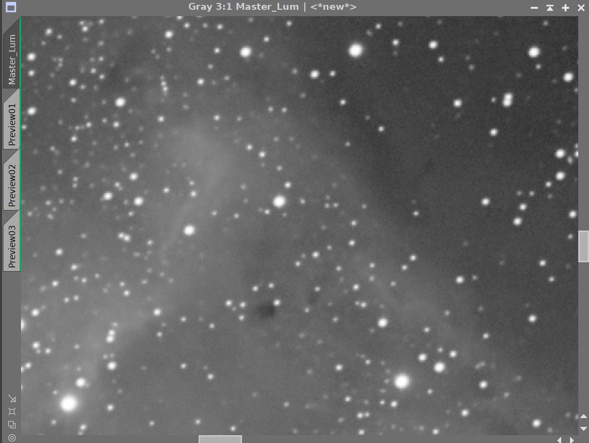
Final Linear Ha (click to enlarge)
Final Linear Lum (click to enlarge)
Final Linear RGB (click to enlarge)
Final Linear Images
10. Take the Ha and Lum Images Nonlinear and Finish Processing
Take the Ha image Nonlinear
Select a preview area on a good sample of the background sky.
Run MaskedStretch
Tweak with CT
Reduce bright areas with HDR_MT with levels= 8
Run a Final CT
Run LHE with Radius = 130, contrast limited = 2.0, Amount = 0.5 and a 10-bit
Take the Lum image Nonlinear
Select a preview area on a good sample of the background sky.
Run MaskedStretch
Tweak with CT
Reduce bright areas with HDR_MT with levels= 6
Run a Final CT
Run LHE with Radius = 130, contrast limited = 2.0, Amount = 0.5 and a 10-bit
Ha Nonlinear Processing
Ha image after MaskedStretch (click to enlarge)
Ha after HDR_MT with level - 8 applied (click to enlarge)
Ha after initial CT to adjust tone scale (click to enlarge)
After LHE and a final CT to reduce overall intensity applied. (click to enlarge)
Lum Nonlinear Processing
Lum Image after MaskedStretch Applied (click to enlarge)
Nonlinear Lum after HDR_MT applied with levels = 6 (click to enlarge)
Nonlinear lum Image after CT applied (click to enlarge)
Nonlinear Lum after LHE and a final CT (click to enlarge)
11. Take the RGB image Nonlinear and Create the LRGB Image
Select a preview of a good sample of the background sky
Run MaskedStretch using the preview above
Run CT to adjust tone and color sat - it should be reasonably dark and saturated in preparation for the L image injection
Copy the Nonlin_RGB image and rename it LRGB
Run LRGBCombo using the Nonlin Lum image and a weight of 0.5 on the lum channel
We now have our LRGB image. We still need to fold in the Ha image, but we don’t want to have it impact the entire image. Instead, we will use it to reinforce the definition of the major areas of nebulosity. To do this, we will use a range mask to focus the integration of the Ha image.
Make Ha range mask with RangeSelect on the nonlin_Ha image to cover the main portion of nebulae.
Apply the mask to the LRGB image.
Use LRGBCombination with Ha - and add it to the LRGB image with a weight on the Ha channel of 0.4
Apply Blanshan Star Reduction
Make a clone of the LHaRGB image
Run starnet2 on it to create the starless image
Apply Blanshan Method V3 with iteration= 2, mode = 3
Run DarkStructureEnhance script with default parameters
Run ColorSaturaton to enhance the blues and the reds.
Nonlin RGB image after MaskedStretch and a CT pass. (click to enlarge)
Final Nonlinear Ha image (click to enlarge)
Final Nonlinear Lum image (clock to enlarge)

Final Nonlinear images: Ha, Lum and RGB
Initial LRGB image after L-insert. (click to enlarge)
LRGB after Ha insertion using a Ha range mask (click to enlarge)
After Blanshan Star Reduction with Method 3 (click to enlarge)

Ha Range Mask (click to enlarge)

Starless image created with Starnet2 - used by the Blanshan Star Reduction Method (click to enlarge)
After DarkStructureEnhance Script run with default parameters (click to enlarge)

Final ColorSaturation curve used to tweak colors

Final image after ColorSaturaton adjustment
12. Export to Photoshop
Save images as Tiff 16-bit unsigned and move to Photoshop
Use Camera Raw Filter to adjust Global Clarity, Texture, and Color Mix
ColorMix is much easier to use to adjust hues in an image compared to the tool provided by Pixinsight, and I tend to do this final operation in PhotoShop
Use a lasso with 150-pixel feather to select the Fist region and use Clarity and Colorix to enhance.
Use StarShrink to reduce just the largest stars further. Add watermarks
Export Clear, Watermarked, and Web-sized jpegs.
The final image
The portable scope platform is supposed to be, well, portable. That means light and compact. In determining how to pack this platform for travel, I realized that the finder scope mounting rings made no sense in this application and I changed them out with something both more rigid and compact - the William Optics 50mm base-slide ring set.