
NGC6995/IC1340 - The Bat Nebula! - 13.9 hours in SHO
Date: Aug 10, 2022
Cosgrove’s Cosmos Catalog ➤#0108
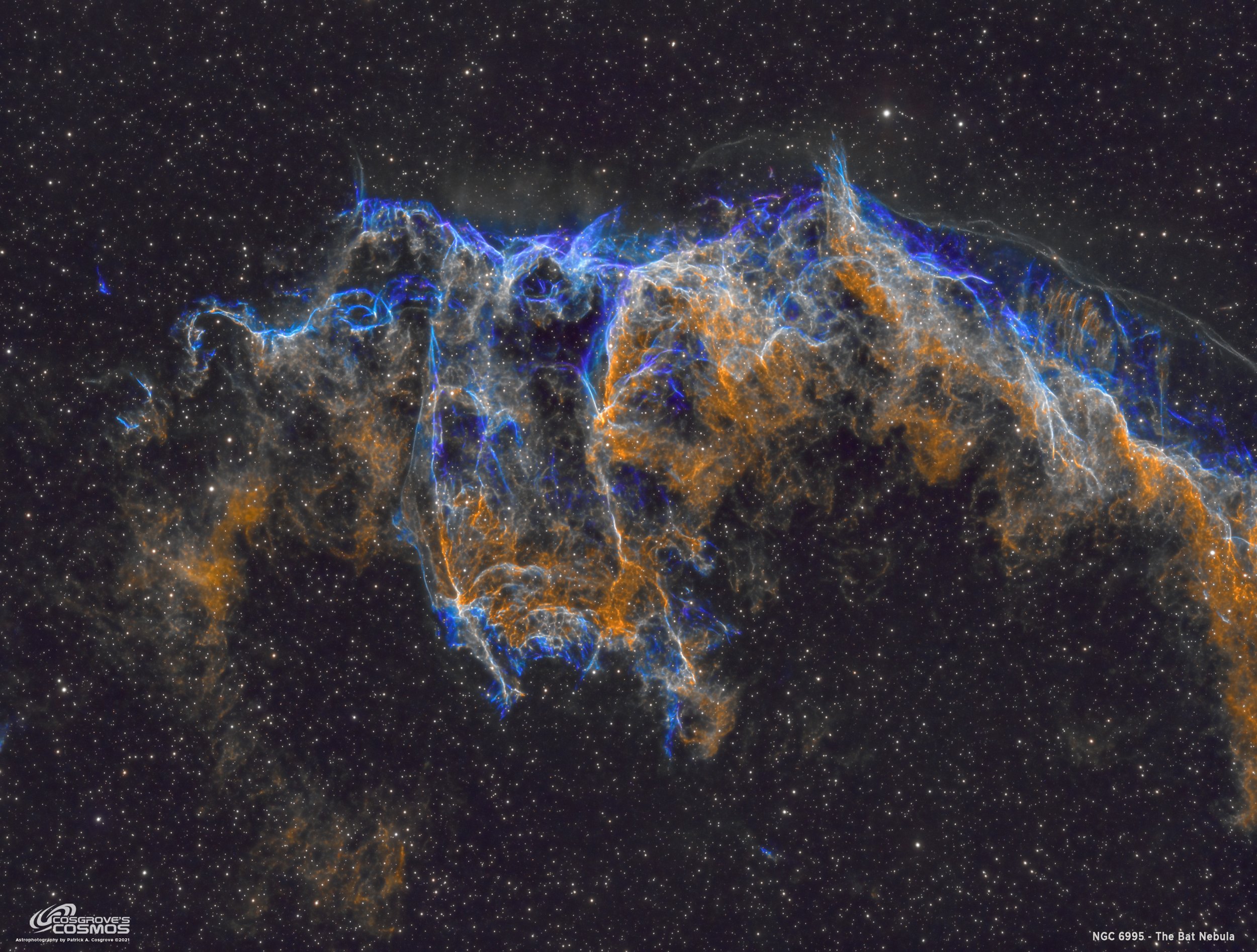
NGC6995/IC1340 - The Bat Nebula - really a small portion of the Eastern Veil Nebula! (click for full resolution version via Astrobin.com)
Table of Contents Show (Click on lines to navigate)
About the Target
The Bat Nebula is an eastern portion of the Veil Nebula, a large supernova remnant that spans 6 degrees of sky in the constellation of Cygnus.
Often referred to as the Cygnus Loop, this Nebula is a great sphere of expanding gas that resulted from a star that was 20 times more massive than our own Sun, which exploded in a supernova some 10-20 thousand years ago. At the time of its explosion, the supernova would have been visible on Earth as being brighter than the planet Venus and would be visible during the day.
Gas ejected in this explosion has been expanding since that time and has evolved to display some complex curved filamentary structures as it is compressed by the shock wave.
As this shell has expanded, it has become visually segmented over time, and each fragment has been identified as a different catalog entry.
The Cycnus loop is located 2,400 light-years away and is large enough to span the equivalent of 12 full moons across the sky! Catalog designations that are associated with the Cygnus Loop include NGC 6960. 6995, 6974, 6970, IC1340, and Caldwell 33/34.
The Veil Nebula was first discovered by Sir William Herschel in September of 1784. He described it as a "Branching nebulosity ... The following part divides into several streams uniting again towards the south."
The Bat Nebula consists of a particular region of the Eastern Veil Nebula that takes on the form of a Bat. While often identified with NGC 6995, IC 1340 is actually more closely associated with the Bat form. The size of the bat form is roughly the size of the full Moon.
This nebula is an emission nebula, which shines with the light of excited Hydrogen, Oxygen, and Sodium. This property makes it very attractive for narrowband imaging, which shows the details of these complex structured molecular clouds.
Like much of the nebulae associated with the Cygnus loop, the Bat Nebula's structure is quite complex with a very filamentary appearance - yet still displays soft shimmering features that make images of this object a feast for the eyes.
The Annotated Image

This annotated image was created in Pixinsight, using the ImageSolver and Annotate Image Scripts.
The Location in the Sky

This finger chart was created in Pixinsight using the FinderChart process.
About the Project
Introduction
Having survived the creation and existence of the first video introduction, I have suffered through the creation of my second. Ok - Still rough and awkward, but I’ll keep working at it…. View at your own risk - you have been warned….
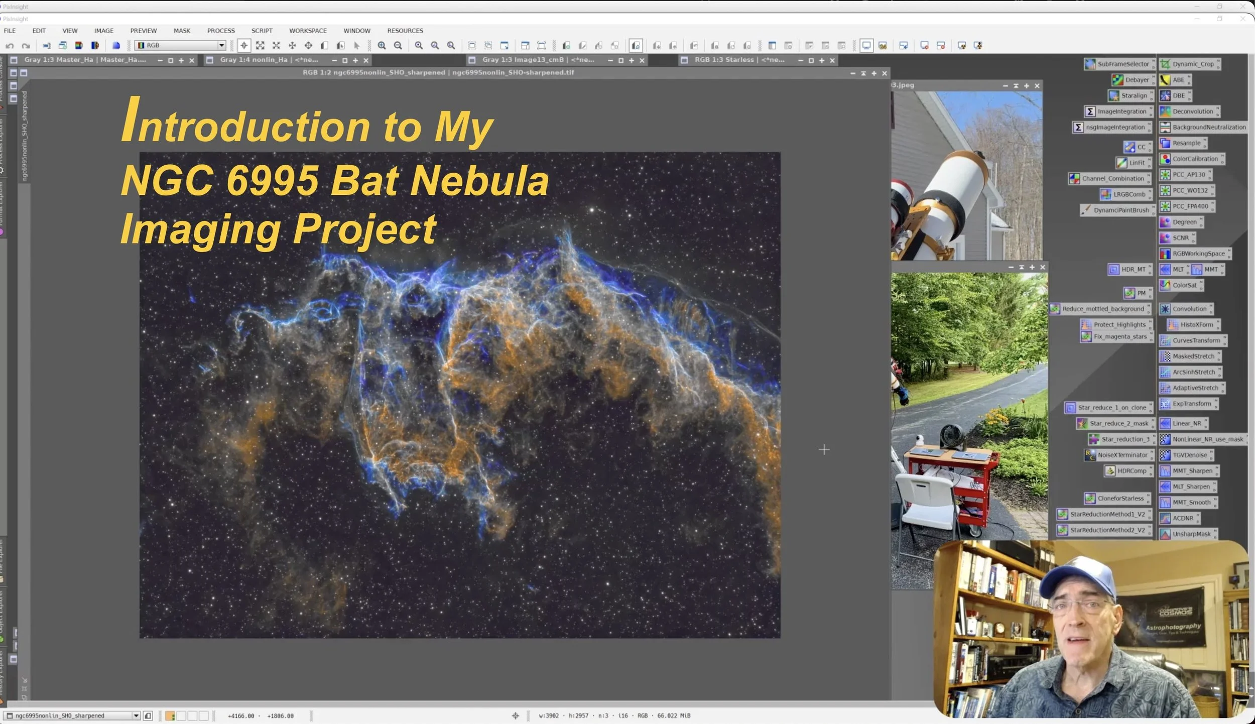
A short video introduction to the NGC 6995 Imaging Project.
Choosing the Target
When I have a clear stretch of weather coming up during a period free of the Moon, I start searching for targets I want to shoot.
Sometimes this is easy.
There may be something on my "want" list that is becoming accessible.
Other times it can be hard.
Based on the characteristic of the target, it gets assigned to one of my three telescopes. Since I have to deal with tree lines, I need to know when the target will rise above the trees and when I can expect to lose the target back into the trees. This predictive element is handled by Stellarium - where I have created a custom landscape view that maps my tree line.
This begins to lay out a simple schedule. But since I can only access a target for about 3 hours a night - I often have unused blocks of telescope time that need to be used. What target can I find to fit into one of those unused time blocks? For this, I must expand my search.
In the case of the Bat Nebula - I was trying to fill the last unassigned block for one of my scopes. The areas of the Veil Nebula were coming into range, but the scale of the nebula was unsuited to the longer 920mm focal length of the scope I was using. Then I came across the Bat Nebula. Hmm - very interesting looking - with lots of complex and yet subtle detail and color! And it has a great size that would work well for that scope. So let’s target that!

Recent NASA photograph of the Cygnus Loop in ultraviolet light, with labels added to point out well known features: The Western Veil (NGC 6960) The Eastern Veil (NGC 6992, NGC 6995, IC 1340) NGC 6974 and NGC 6979 along the northern edge Pickering's Triangle The Southestern Knot, a prominent X-ray feature
And that is how I ended up choosing this Target.
Previous Efforts
I actually have shot the Bat Nebula before. Well, not the Bat Nebula, as much as its parent structure. In July 2020, I shot the entire Veil Nebula in narrowband for the very first time.
That image posting can be seen HERE.
But I will show it here as well:
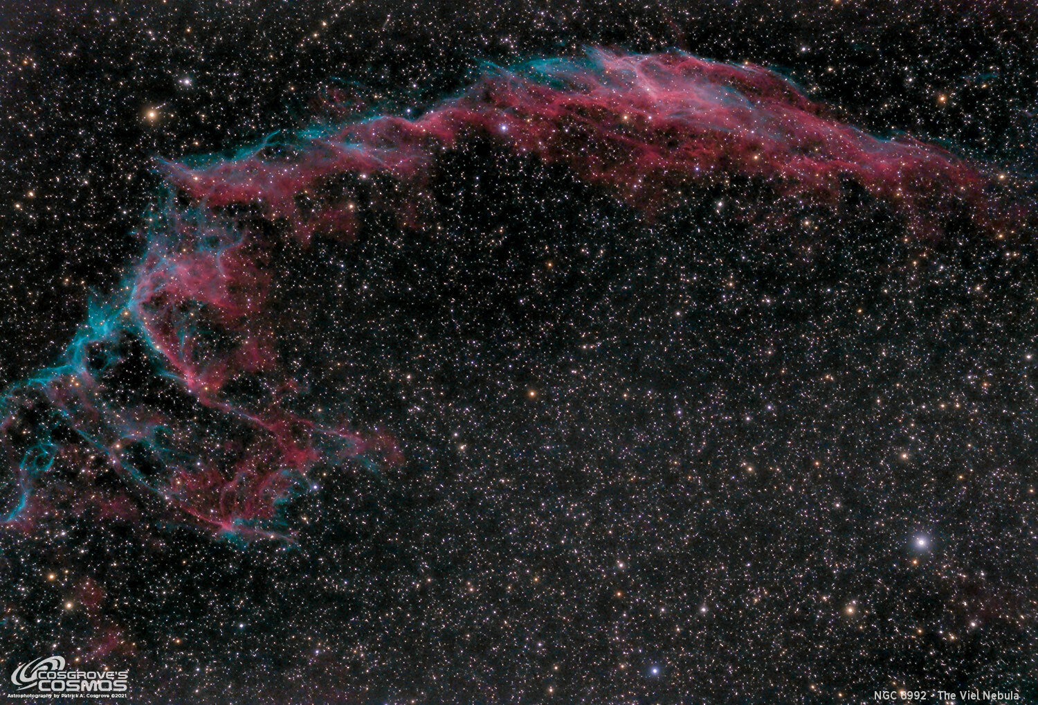
My first version of the Veil Nebula - NGC 6992 - was shot back in July of 2020. The Bat Nebula can be seen towards the extreme left side of the image.
Can you see the Bat Nebula over on the left side of the image? This helps put things into context. This particular image came out pretty well, I thought - but now my mission was to see if I could produce a higher level of quality from the same section of sky.
By the way - I think that is a very common theme in target selection for astrophotographers.
It often seems as though astrophotographers fall into one of the buckets below when trying to find a target:
The SightSeer. You are new to astrophotography, and you chase after all of the most famous targets that had meaning for you from your visual observing days. It's like having those National Park Passports they give kids - so they can get them stamped as their families visit each new park.
Let Me Try That Again! This is super popular. You shoot some things every year, because since the last time you shot it, you got a new scope, or new camera, or learned some new processing techniques, or because you are naturally smarter and more handsome than last time, so why not prove it by sotting it again and then showing everyone who will listen how much better you are now. Not that I do that or anything. (Did you notice my old image of the Veil? Well, this one is so much better…).
Plowing New Ground. Shooting something not as well known - something different that will stand out from the pack.
Going to Extremes. Super long integrations, 14 filter sequences, super long sub times. Or the other end, super short.
There are probably some other themes here, but I digress. This image is certainly from category #2 above!
Data Capture
If I am very lucky, I will get 3 clear nights in a row during a moon-free period. I rarely get more than that. I have had four-night stretches. This time around, we had five nights of great weather! - cool nights, clear skies, and no bugs! What is not to love?
Many images of the Bat Nebula that I have seen were Bi-Color - in other words, only two narrowband channels were collected, and these were mapped onto a Red, Green, and Blue channel to form a color image. These images can have dramatic red-blue colors and can be quite impressive. But everything I have read suggested that this region has good signals in all three narrowband channels (Ha, O3, & S2), so why not collect them all and see what we can get?
So for five nights, I captured data with little difficulty. I also grabbed flats calibration shots for three of the five nights. For the last two nights, I was too sleep-deprived even to care - so I did get a little sloppy here.
At the end of the five nights, I had a lot of data on four different targets. This is the second target I have processed and published of the lot.
Data Analysis
Blink analysis showed generally good subs with only two frames in total removed for cloud issues.
SubFrameSelector analysis also showed generally good frames, but 21 frames were removed before ImageIntegration because they had FWHM or Eccentricity measures that were out of line. This means that the total integration of 15.7 was reduced by 1.75 hours.
With narrowband subs being 5 minutes long, it hurts to have many subs eliminated! But I have found that the stacking process is very much a garbage-in/garbage-out kind of a deal. It does not help your final result if you are leaving images that have bloated stars or egg-shaped stars from tracking issues. Sometimes the rejection logic will minimize the impact of such frames - but the more you have that are like that, the less likely it is that rejection will be able to deal with it.
It’s best to remove the offending frames before you run integration!
When I am working on a small galaxy or planetary nebula, I can get very aggressive about this. For this image, where fine detail was less critical, I was only mediumly aggressive about it.
Image Processing
For the most part, I followed my current standard SHO processing workflow.
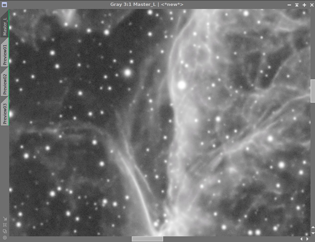
I created a synthetic Luminance image by using ImageIntegration to add together the Ha, O3, and S2 master images. This image was then deconvolved and processed - to be later combined with a simple SHO color image. The L image is processed for peak sharpness and detail. The color image is processed for good color and low noise. These are then combined with LRGBCombination, and we end up with the best of both worlds.
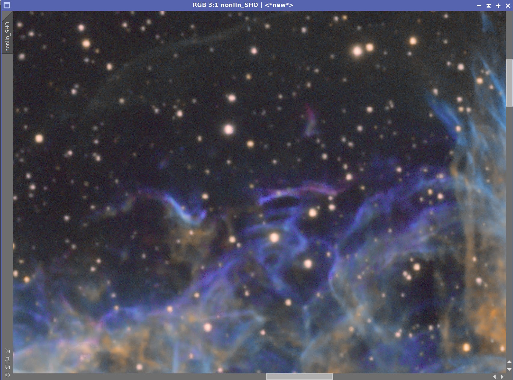
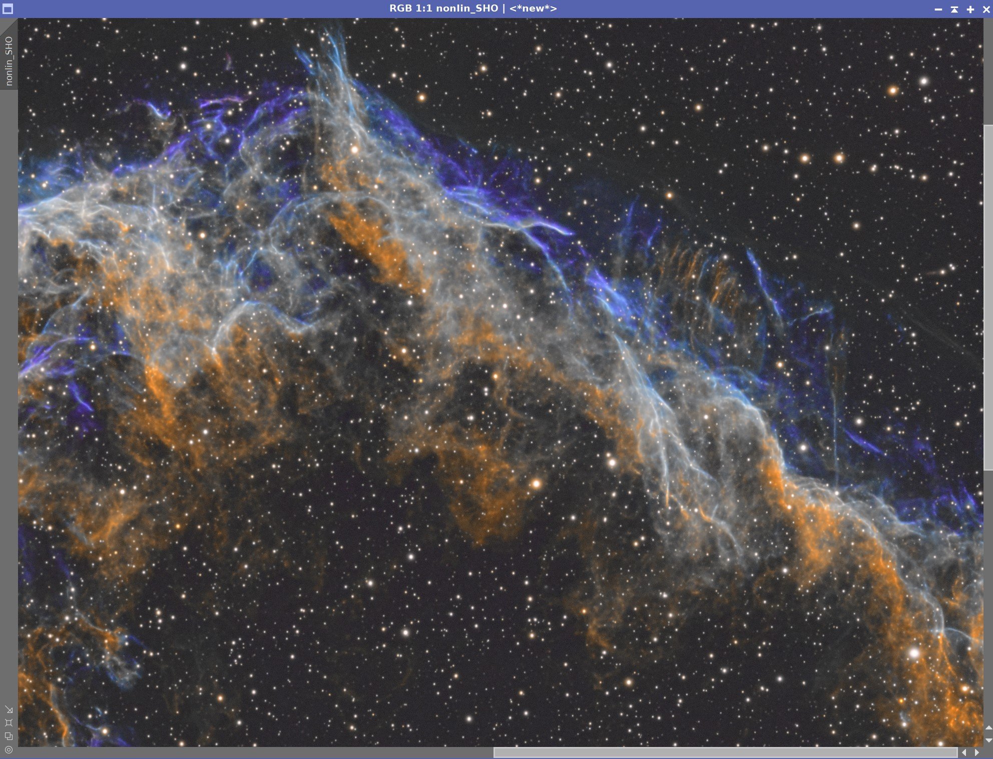
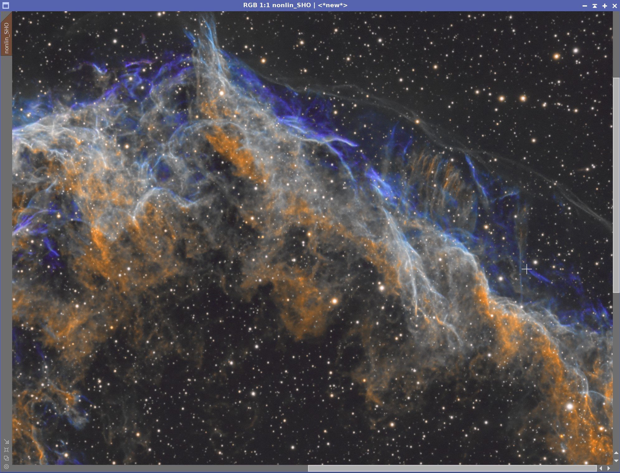
On the right side of this image, there are some beautiful shimmering details that I really like.
The trouble was that I could see these features in the color image but not in the synthetic L image. When I inserted the L image, I lost this shimmering detail. This was not acceptable.
So I tried something I have not done before.
The detail in question was on the lower end of the tone scale. So I created a range mask that covered the medium and high end of the tone scale. I applied this to the SHO image and then folded the L image into the SHO image with LRGBCombine, and I got the shimmering detail and the sharpness for the higher end of the tone scale while protecting the shimmering detail in the lower end of the tone scale. This worked to my satisfaction.
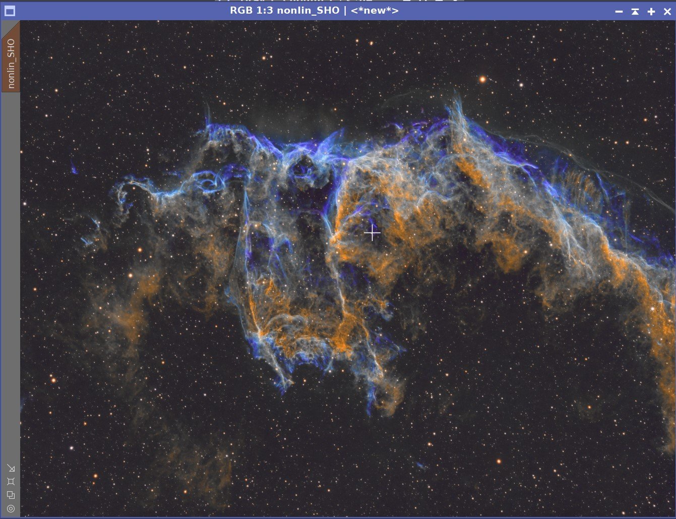
Discussion of Results
I was very pleased with my final result. This is a complex and chaotic area of space, the image captures and highlights this. On one hand, I found I could lose myself in the details. Scrolling through the image at full resolution is a real experience! Some many interesting details to be seen!
On the other hand, sending hours processing this image does seem to cause eye fatigue. I get worn out working on it for too long! So much is going on!
A detailed Processing Walk-Through is provided for this image at the end of the posting…
More Information
Wikipedia: The Cygnus Loop
Wikipedia: The Viel Nebula
Science.nasa.gov: The Bat Nebula
Capture Details
Lights Frames
Data was collected over five nights: July 28,-July 31, and Aug 2.
Number of subs after Blink and SubFrameSelector analysis and removal
50 x 300 seconds, bin 1x1 @ -15C, Gain Zero, Astrodon 5nm Ha
60 x 300 seconds, bin 1x1 @ -15C, Gain Zero, Astrodon 5nm O3
57 x 300 seconds, bin 1x1 @ -15C, Gain Zero, Astronomiks 6mm S2
Total of 13.9 hours
Cal Frames
25 Darks at 300 seconds, bin 1x1, -15C, gain Zero
12 Flats at bin 1x1, -15C, gain Zero - for Ha, O3, S2 filters
25 Dark Flats at Flat exposure times, bin 1x1, -15C, gain unity
Software
Capture Software: PHD2 Guider, Sequence Generator Pro controller
Image Processing: Pixinsight, Photoshop - assisted by Coffee, extensive processing indecision and second-guessing, editor regret, and much swearing…..
Capture Hardware:
Scope: William Optics 132mm f/7 FLT APO Refractor
Focus Motor: Pegasus Astro Focus Cube 2
Cam Rotator: Pegasus Astro Falcon
Guide Scope: Sharpstar 61EDPHII
Guide Focus Motor: ZWO EAF
Mount: Ioptron CEM 60
Tripod: Ioptron Tri-Pier
Camera: ZWO ASI1600MM-Pro
Filter Wheel: ZWO EFW 1.2 5 x8
Filters: ZWO Gen II 1.25” LRGB,
Astrodon 5nm Ha & O3 filters
Astronomiks 6nm S2 filer
Guide Camera: ZWO ASI290MM-Mini
Dew Strips: Dew-Not Heater strips: Main & Guide Scopes
Power Dist: Pegasus Astro Pocket Powerbox
USB Dist: Startech 8 slot USB 3.0 Hub
Polar Align Cam: Polemaster
Software:
Capture Software: PHD2 Guider, Sequence Generator Pro controller
Image Processing: Pixinsight, Photoshop - assisted by Coffee, extensive processing indecision and second-guessing, editor regret and much swearing…..
Click below to see the Telescope Platform version used for this image
Image Processing Walk-Through
(All Processing done in Pixinsight - with some final touches done in Photoshop)
1. Blink Screening Process
Ha
Some slight gradients
Very few trails
No frames removed
O3
Some gradients
One plane!
Very few trails
One frame was removed for cloud obstruction
S2
Some trails
Some gradients
Seems like chunks with some slight attenuation from thin clouds - leave in for now - evaluate with subframe selector later
Remove one frame from heavier clouds
Flats
collected for the first 3 nights. Data looks good
Dark flats
collected for the first night - data looks good
Darks
Get 300-second Darks from the 7-26-22 cal files.
Below you can see videos of the Blick runs. Note that at the end of each video, you can see a “+” symbol curving across the screen - this is an artifact of the screen recording mode when I moved the cursor to stop the recording.
2. WBPP 2.4.5
Reset everything
Load all lights
Load all flats
Load all darks
Add the “Night” keyword
Select - maximum quality
Reg reference - auto - the default
Select output directory
Enable CC for all light frames
Pedastal value - auto for all light frames
Darks -set exposure tolerance to 0
Deselect integration mode - just cal and alignment
Map flats and darks across nights
Ran wth no problems in about 30 minutes

WBPP Calibration view.

Post Calibration View.
3.0 Use SubFrameSelector to analyze the Calibrated subs
After WBPP ran, I used SubFrameSelector to check the quality of my subs.
Subs for each filter were loaded into the tool, and metrics were computed. FWHM and Eccentricity were the key metrics I used in this analysis. Screenshots for each filter are attached below.
Ha images: 7 deleted for having too high an FWHM or Eccentricity value
O3 images: 6 deleted for having too high an FWHM or Eccentricity value
S2 images: 8 deleted for having too high an FWHM or Eccentricity value
I was not very aggressive in what I eliminated for this image, as peak resolution was not my goal. A total of 1.7 hours of integration was thus lost.

Ha Sub FWHM - Note eliminated frames

O3 Sub FWHM - Note eliminated frames

S2 Sub FWHM - Note eliminated frames

Ha Sub Eccentricity - Note eliminated frames

O3 Sub Eccentricity - Note eliminated frames

S2 Sub Eccentricity - Note eliminated frames
4. Integration
ImageIntegration
ImageIntegration was run for each Master image.
It used the same setup for each run.
ESD was chosen for rejection.
Large scale rejection checked - 2x2
A sample panel for ImageIntegration can be seen below
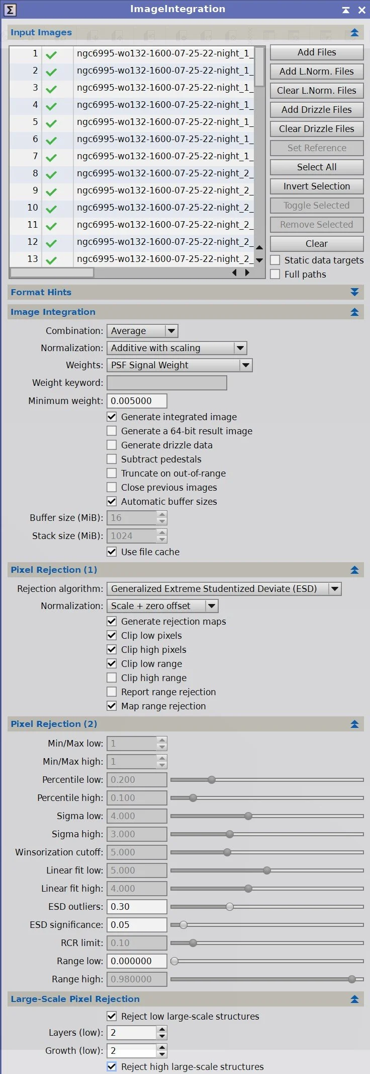
ImageIntegration panel settings.
Rejection High - Ha: Note trails removed (click to enlarge)

Rejection High - S2: Note trails removed (click to enlarge)
Rejection High - O3: Note trails removed (click to enlarge)
5. Crop all of the images
A common crop level was selected, and DynamicCrop was used to trim all of the master frames.
A crop used is shown below:

The crop used for this image.
6. Dynamic Background Extraction
DBE was run for each image using the subtraction method. Below are the Sampling plans, the before image, the after image, and the removed background images.
Note - very little nonuniformities seen.
DBE: Ha Sampling (Click to enlarge)
DBE: O3 Image Sampling (Click to enlarge)
DBE: GS2 Sampling (Click to enlarge)
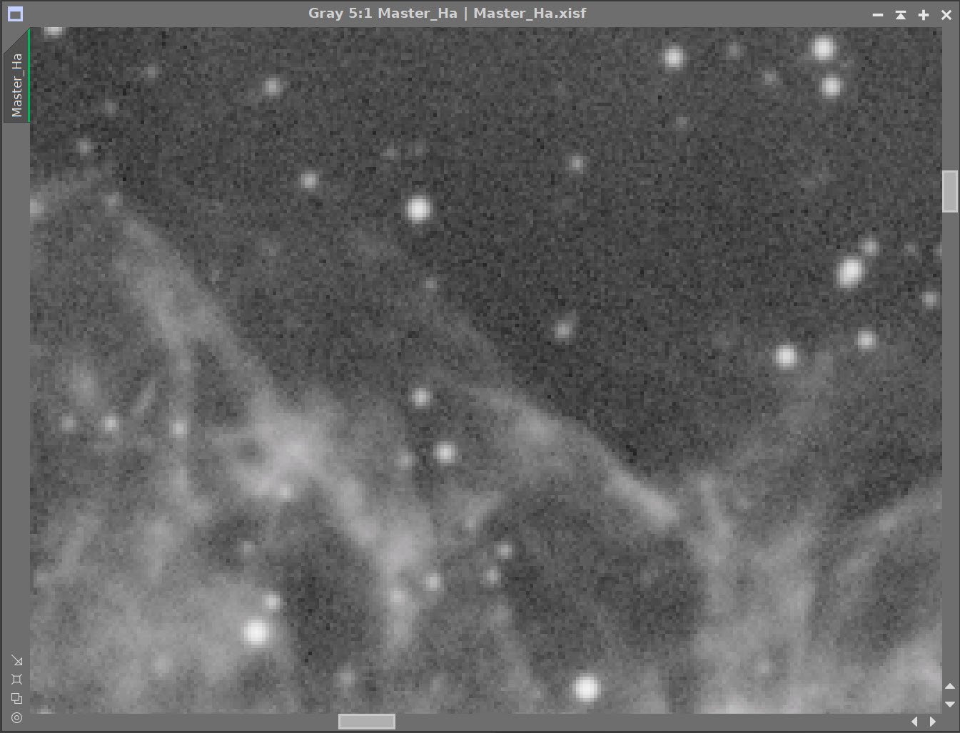
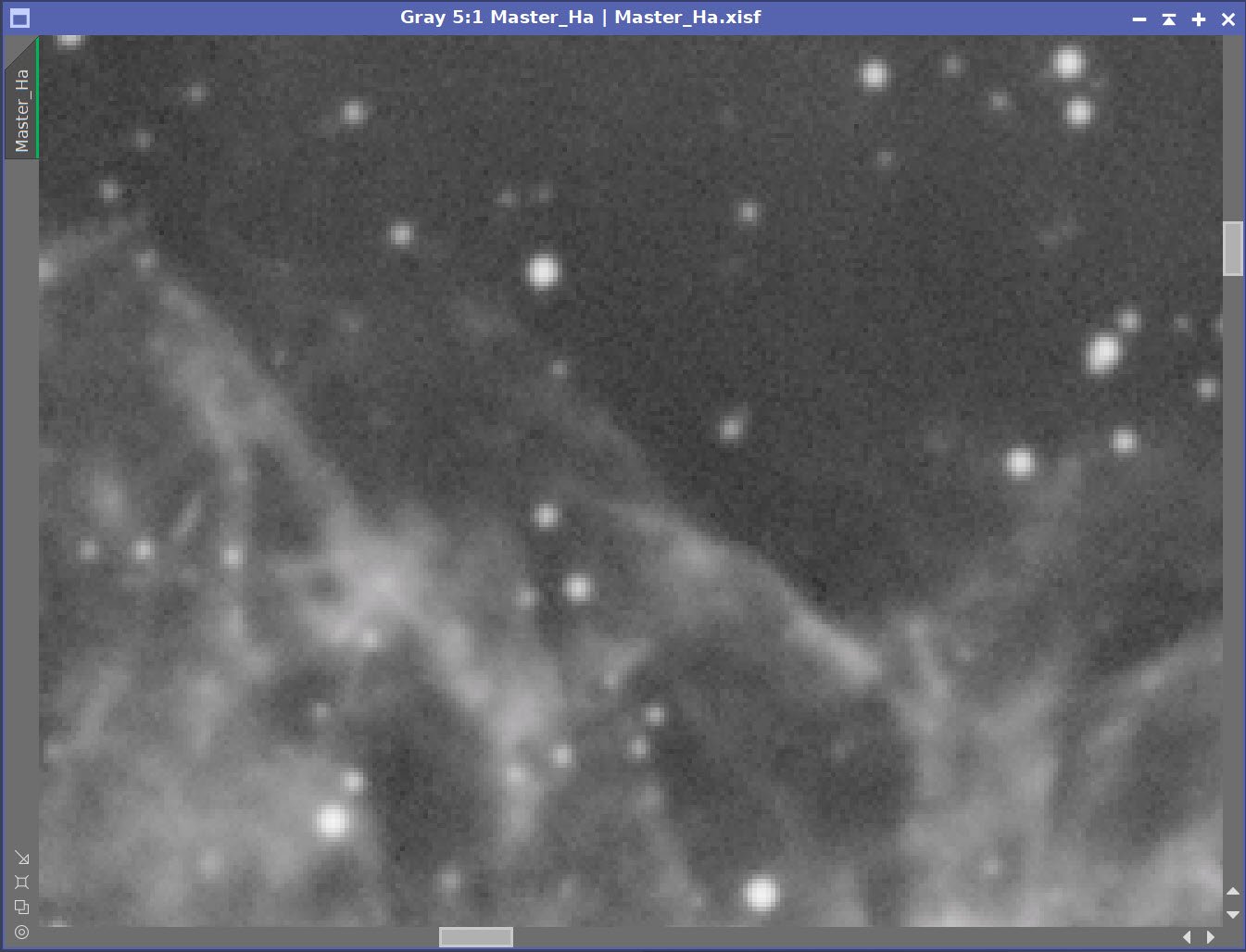
Ha image Before DBE (click to enlarge)
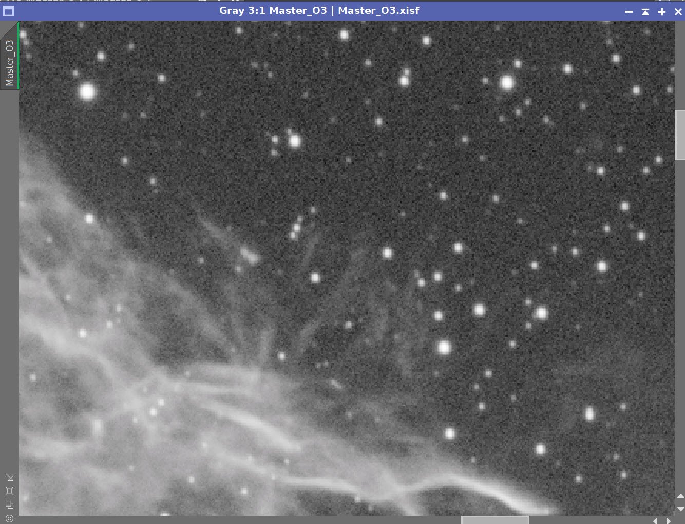
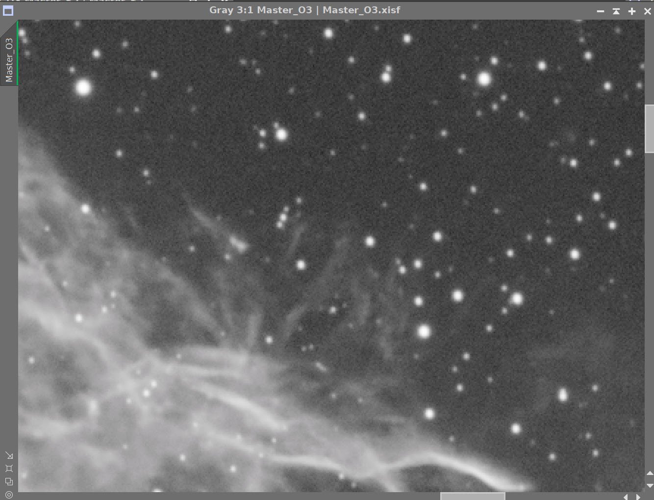
O3 Image Before DBE (click to enlarge)
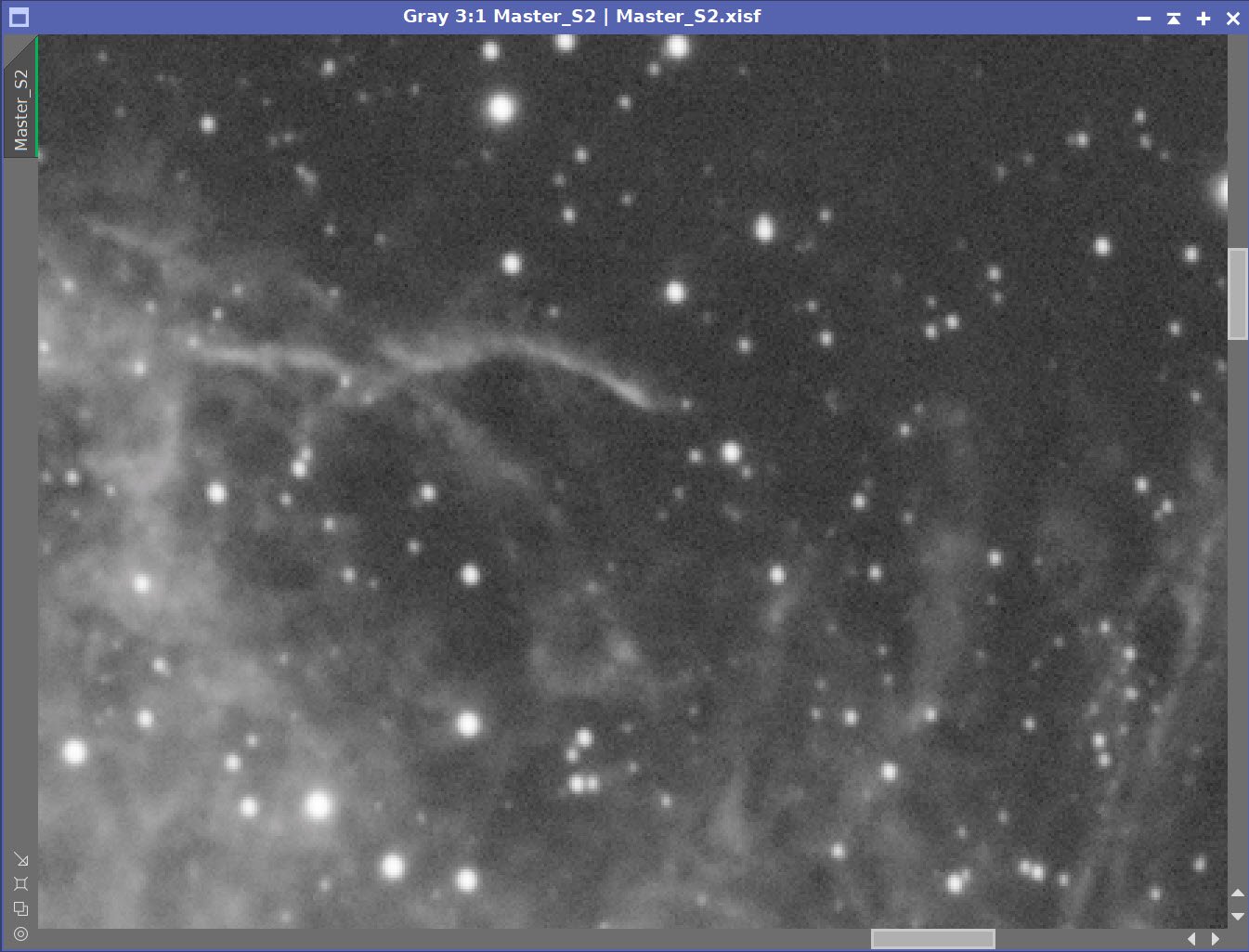
S2 image Before DBE (click to enlarge)
Ha image After DBE (click to enlarge)
O3 Image After DBE (click to enlarge)
S2 Image After DBE (click to enlarge)
Ha background removed (click to enlarge)
O3 background removed (click to enlarge)
S2 background removed (click to enlarge)
7. Create and Process the Linear Color Images
After Crop and DBE, the only other thing I do on the color masters before going nonlinear is to do some light noise reduction to “Knock the fizz off”
This is done by running Noise XTerminator with a value of 0.5

Before and After application of RC Noise XTerminator with a value of 0.5
For Ha, O3, and S2 Linear Images
8. Create a Synthetic Luminance Image and complete its Linear Processing
Write out master Ha, O3, and S2 images as files (needed for the next integration step)
Run ImageIntegration
load the master Ha, O3, and S2 files
Default integration method
No rejection methods
Run - creating the Master L file
Prep for Deconvolution
Create a PFS-Lum image by running PFSImage Script
Create LDSI image
Run the Starmask process with parameters seen in the screen snap below
Run HT to boost the resulting star mask using the HT curve seen in the snap below
Select a few image previews for testing deconvolution parameters
Run Deconvolution using the PFS image and the LDSI Image - iteratively test parameters until the best result is obtained.
see final parameters below.
Run Noise XTerminator with a value of 0.5
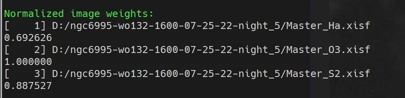
The relative weights applied by ImageIntegration to the 3 input files to create the Synthetic Lum image. ote how strong the O3 and S2 contributions are!

PSFImage Panel for the Lum image.

The Lum PSF image

Stramsk setting used to create original LDSI map

HT transform to boost LDSI map

The final Lum LDSI image.

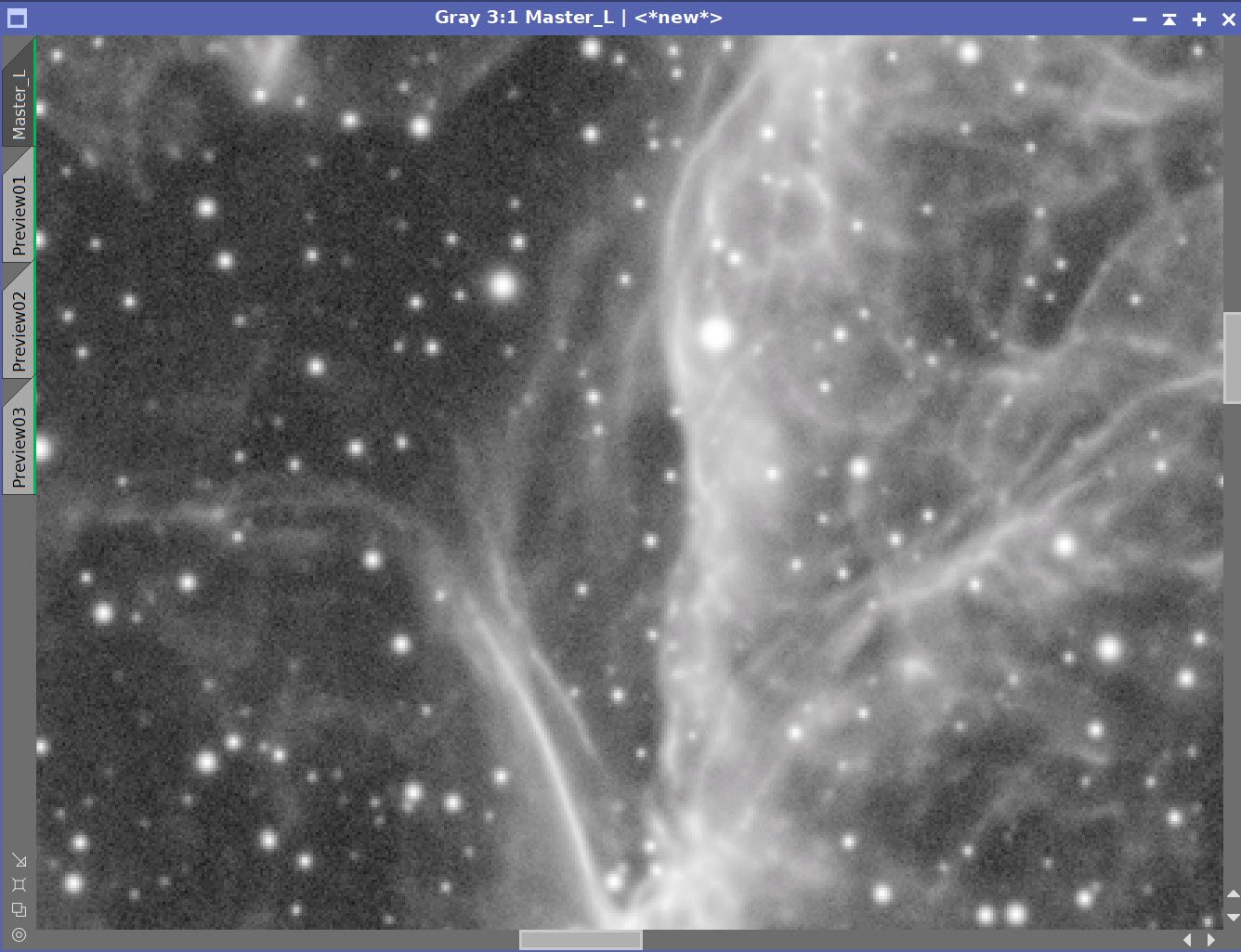
The three preview regions set up to explore decon settings for the Lum image
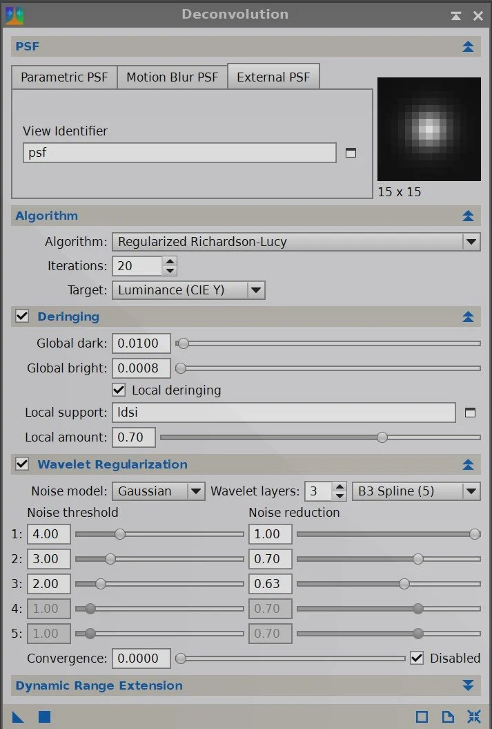
The final settings on the Decon Panel for the Lum image.

Lum Image Before and After Deconvolution, and After Noise XTerminator 0.5
9. Take the Lum Nonlinear and Finish Processing
Go nonlinear using the STF->HT method.
Run CT and adjust tone scale
Run LHE with radius = 32, contrast limit = 2, Amount = 0.5, and 8-bit histogram
Final CT tweak
Lum image after MaskedStretch (click to enlarge)
Lum after LHE applied (click to enlarge)
Lum after CRT to adjust tone scale (click to enlarge)
After final CT (click to enlarge)
10. Create the Initial Color SHO Image and Process it.
For each color image
Select a Preview of the background image
Run MaskedStretch using the Preview above
Balance colors images using LinFit, using Ha as the master Image
Create the first color SHO image with the ChannelCombination tool
Run SXNR to remove the green balance
Create a set of color masks using the ColorMask Script
Magenta
Blue
Apply the Magenta Color Mask
Use CT to reduce Saturation at both low and high points, and increase the neutral tone scale
Apply the Blue Color Mask
Use CT to lighten the tone scale, boost color
With RangeSelection, create a background mask
Apply background mask
Use CT to reduce saturation and darken the background
Remove mask
Run Noise XTerminator with a value of 0.6
Run ColorSaturatin and boost blues, greens, and yellows

FInal Ha, O3, and S2 image prior to the creation of the first SHO image
Initial SHO image (click to enlarge)

Magenta Mask
After using SCNR to remove the green balance (click to enlarge)

Yellow Mask

Blue Mask

Background Mask

CT Adjustment with Magenta Mask in Place

After CT adjustment with the Background Mask in place

After CT adjustment with Yellow Mask in place
SHO Image - Before and After Noise XTerminator 0.6

ColorSaturation Process Panel Settings

After ColorSatruation Adjustment

SHO Color Image after one final CT adjustment.
11. Integration of the Lum Image to the SHO Color Image
Use LRGBCOombination to fold the Final L image into the SHO image
REsults are concerning ! I am loosing detail on the shimmering elements of the nebula

Final L image.

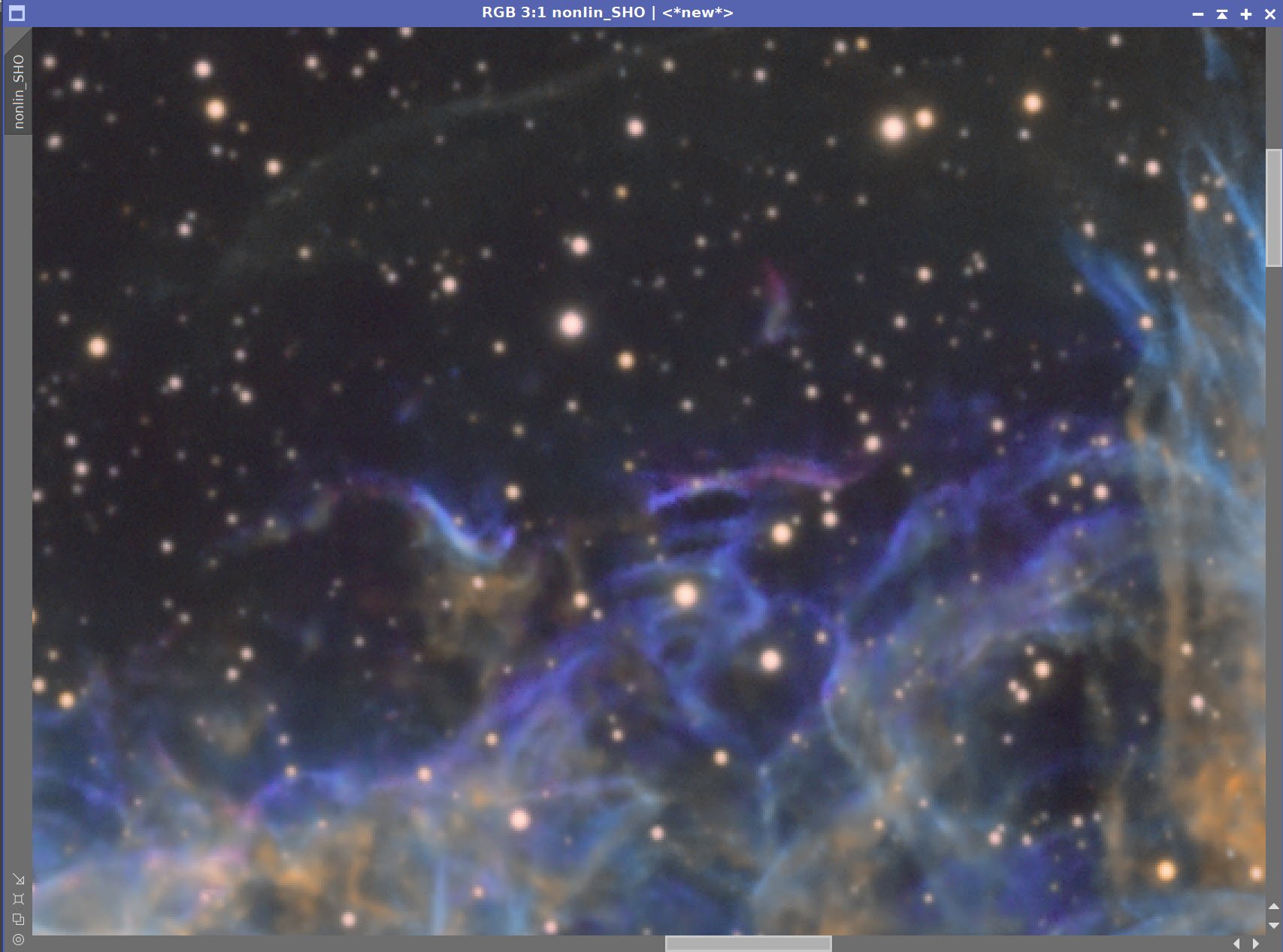
Final SHO image.

After L-Insertion - Note that the shimmering details in the upper left quadrant were muted! This is because this detail was missing in the Synthetic L image. To fix it, we need to redo this step with a mask that only allows the L-Insertion to affect mid and high-range values.
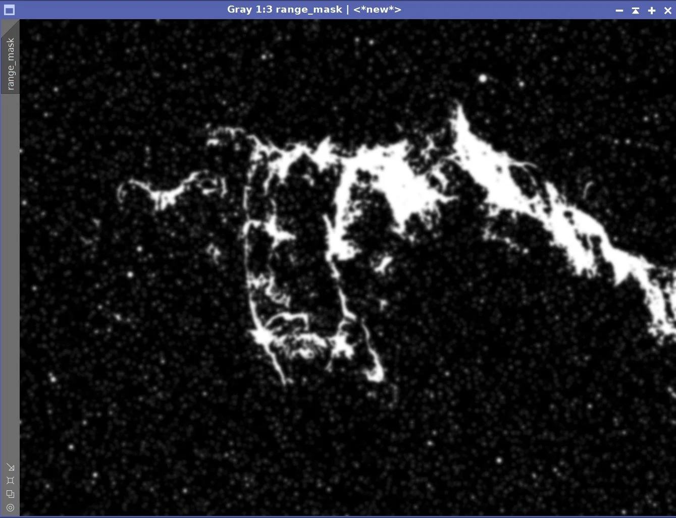
Here is the Range Mask - note that no trace of the shimmering feature is seen in this mask. It is therefore protected.
LRGBCombination used to insert L data - With and Without the Protective Range Mask

The FInal Image after a final CT adjustment.
12. Star Reduction
My last project caused me to try out the new Star Reduction Methods developed by Bill Blanshan. I was impressed with his tools, and so I wanted to use them again on this project.
Drag the CloneforStarless Process icon onto the image
Run Starnet2 on the resulting clone image
Run StrRecutionMethod3_V2 on the image using Iteration = 1 and Mode=1
Bils Process Icons once installed.

The starless Image created for supporting the Star Reduction tool.

Before Star Rection (click to enlarge)
After Star Reduction
13. Star Adjustment
At this point, I noticed that most of the stars had an orange cast to them. When you are doing narrowband imaging, often the best you can hope for is white stars - or you need to plan in advance to replace these stars with RGB stars you have captured in their own exposure sequences.
My solution here was to create a star mask and use it to target the stars I wanted to desaturate.
Create the Star Mask
Using pixel math, subtract the starless image from the original image.
Now extract a neutral image from this color star image
Use Binarize to clip the resulting star images
Use Morphalogicaltransform with a 5x5 circle pattern and dilate the image one time.
Run Convolution with the StdDev set to 2.0
Apply the star mask and invert it
Run CT and lower the saturation for the brighter portion of the tone scale.

The Star Mask Created
With the “Orange Stars” (click to enlarge)
After Star Desaturation (click to enlarge)
14. Sharpening
At this point in the process, I shared this version of the image with two local Astrophotographers: Dan Kuchta and Gary Opitz. Dan liked the way it looked, and so did Gary, but Gary took the jpeg and applied some sharpening to it. He thought that it took sharpening well, and shared the result with me. He was right - some sharpening was helpful!
Now in the past, I have been a little gunshy on final stage sharpening because it often seemed to screw up my stars. But this time, I returned to my workstation and applied the Starmask I had already created and then ran MLT with the sharpening parameters shown below. I was pleased with the result!


The Final sharpened image!
15. Export to Photoshop
Save images as Tiff 16-bit unsigned and move to Photoshop
Use Camera Raw Filter to adjust Global Clarity, Texture, and Color Mix
ColorMix is much easier to use to adjust hues in an image compared to the tool provided by Pixinsight, and I tend to do this final operation in PhotoShop
Use StarShrink to reduce just the largest stars further. This further helps the bloat.
Add watermarks
Export Clear, Watermarked, and Web-sized jpegs.
The final image1
I was very excited to get the ZWO ASI2600MM-Pro camera a while back. I ordered it when it was announced and then prepared to wait a long time to get it. When I did get it - I decided to put it onto the AP130 platform. That meant that I could move the ZWO ASI1600MM-Pro, along with its filter wheel over to my William Optics Platform. This now means that all of the platforms have been moved over to a mono camera and my ZWOASI924MC-Pro is now not in use.