
SH2-114 -The Flying Dragon Nebula - a VERY Faint Challenge Target - 17.5 hours HSSrgb
Date: September 7, 2022
Cosgrove’s Cosmos Catalog ➤#0110
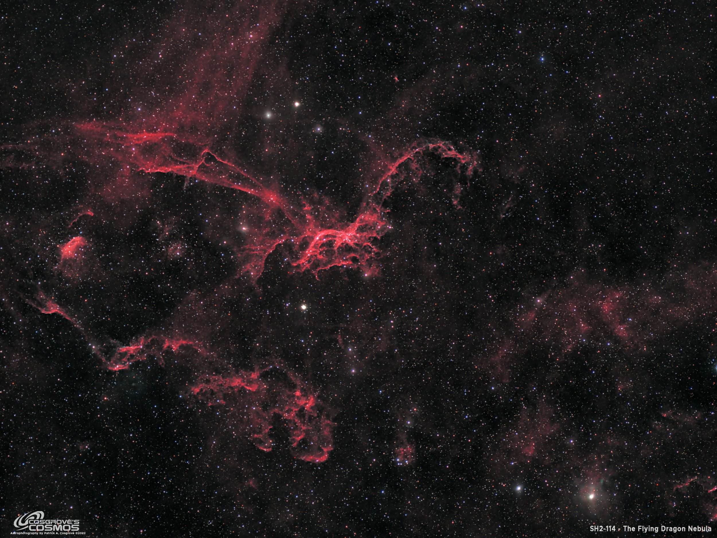
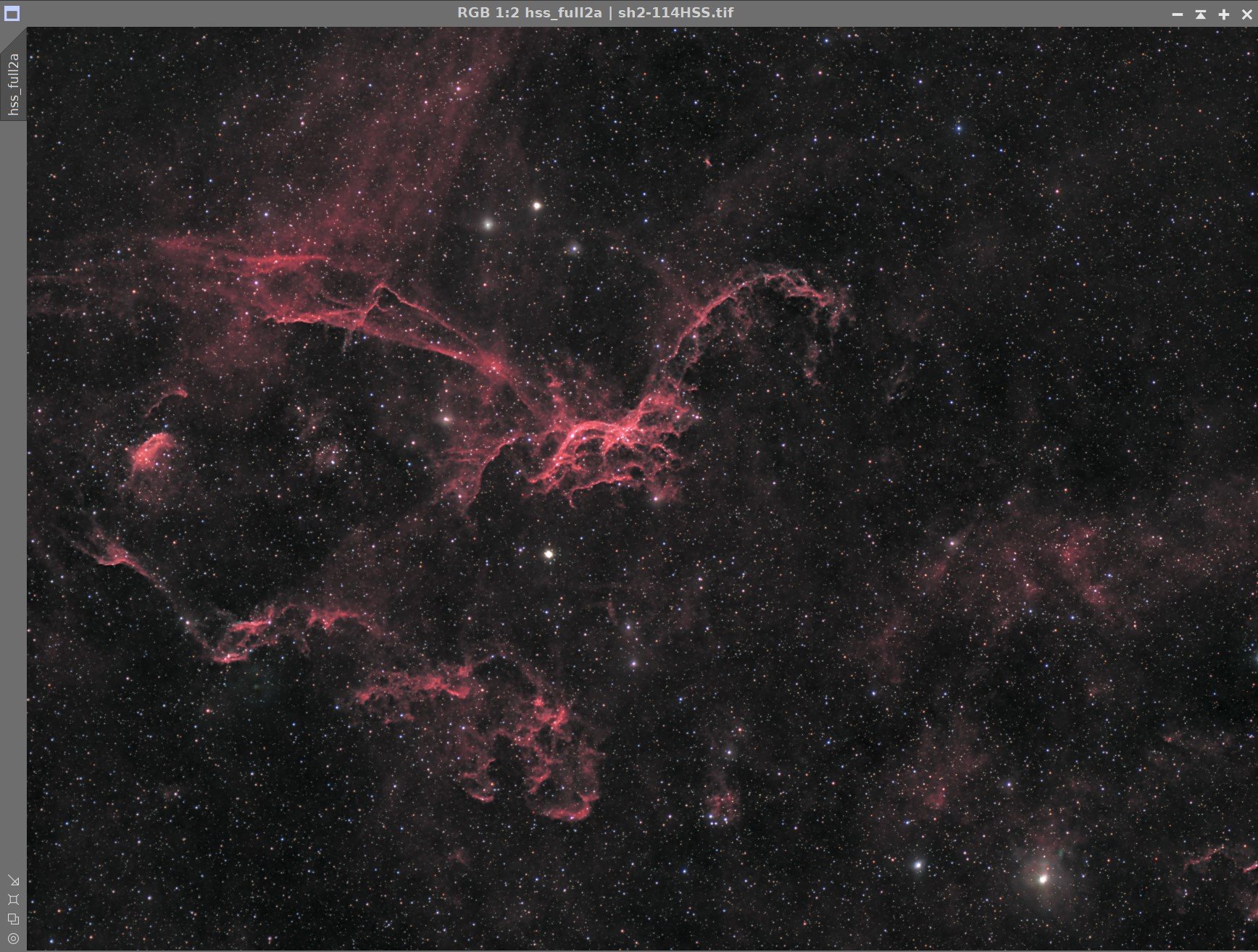
Sh2-114 is a super faint H2 emission nebula in Cygnus, whose form looks like the sweeping wings of a flying dragon! (Click for the full-resolution version via Astrobin.com)

Flickr granted this image Explore Status on Sept 7, 2022!
Table of Contents Show (Click on lines to navigate)
About the Target
SH2-114, better known as the “Flying Dragon Nebula,” is a very faint H2 emission nebula in the constellation of Cygnus. Also cataloged as LBN 347, it is part of a larger complex that includes SH2-113. I have also heard this called the “Red Dragon Nebula.”
This large curving filamentary structure appears to be part of a supernova, but no supernova remnant has yet been identified as the source. The shape of the nebula is most often seen as a winged dragon or bat. This structure seems to have been formed by a combination of intense stellar winds emitted by massive, hot, O and B stars interacting with magnetic fields within the interstellar medium.
Other than this - not much more is known about this object. It is certainly not a common target for Astrophotography and is too faint for visual observation.
Directly above the right wing, halfway between the wing and the edge of the frame, is a planetary nebula. This is cataloged as Kronberger (Kn) 26, and it is a bipolar emission nebula (note: this is not shown on the annotated version of the image)
The Annotated Image

This annotated image was created using Pixinsight’s ImageSolve and AnnotateImage Scripts.
The Location in the Sky

This Finder Chart was created using Pixinsight’s ImageSolve and FindinggChart scripts.
About the Project
Introduction
Below is my video overview of this imaging project.
(Note: These videos are hosted on my just-starting YouTube page as I painfully learn more about how to do video content. Your support and patience are valued and appreciated as I go through this learning curve. I would very much appreciate it if you would subscribe and “ring the bell” on my Youtube Channel, which will greatly help to establish it! Your feedback and suggestions would also help as strive to make this video content better!)
Choosing the Target
I have been working on this project for a while now. I first started collecting data back in late July of this year.
When selecting targets back then, I looked at what was coming up past my eastern tree line, I saw that constellation Cygnus was well placed just past midnight. Cygnus is such a rich area of the Milky Way, and I felt sure I could find an interesting target there.
So I did what I often do when looking for inspiration - I went to Astrobin.com and searched for award-winning images in Cygnus. As I went through the search results, I saw images of the Flying Dragon Nebula that I had not seen before. Designated SH2-114 - this object intrigued me because I was completely unfamiliar with it.
I noted that most images were done in narrowband, and most of the signal was in the Ha channel. I also noted that in most of the images I was on Astrobin - the total integration times were quite long. This suggested that this was a very faint object and should have been a red flag for me - since my ability get capture long integration times is quite limited by my location and site circumstances. Even still - I wanted to give this challenge a go!
Because of the size and scale of the target and the fact it was very faint, I decided to use my Askar FRA400 telescope platform for this capture. This would give me the widest field and the fastest optics of any of the scopes I am now using.
Data Capture
To kick the project off, I started by capturing a 5-minute sub for the Ha, O3, and S2 filters. I wanted to get a feel for what signal levels I would be dealing with. I was shocked to see a very little signal for Ha, a barely noticeable signal on S2, and I saw virtually nothing on O3. based on these results, I decided to capture just Ha and S2 data, thinking I could do some form of B-Color image with an HSS blend.
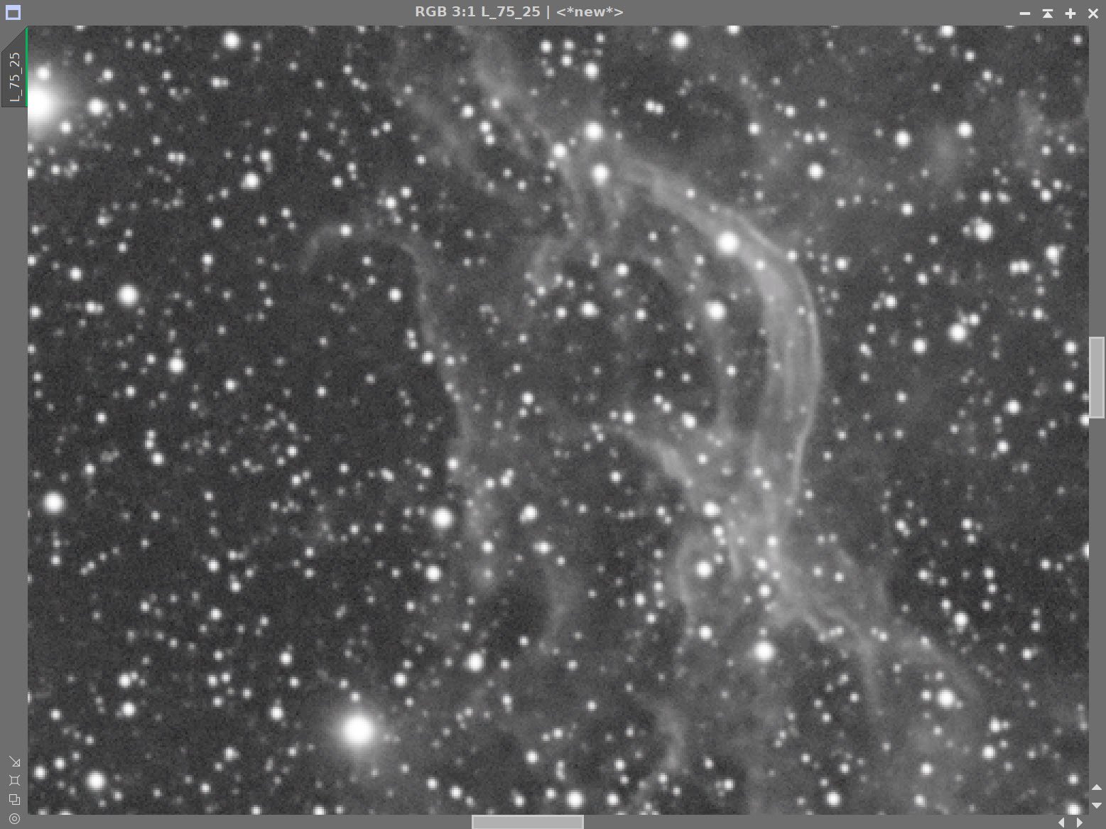
This is a single 5-minute Ha Sub. The nebula barely shows! (click to enlarge)
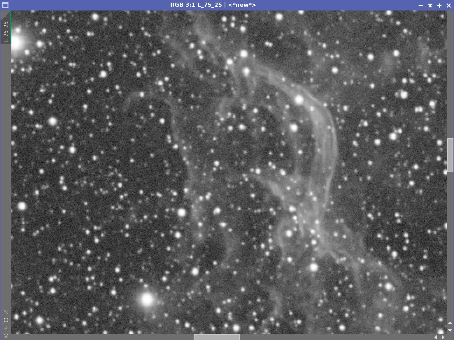
This is the same Ha sub - only now zoomed in on the brightest part of the nebula. Incredibly faint!! (click to enlarge)
This is a single 5-minute S2 Sub. The nebula barely shows! (click to enlarge)
The same for the S2 sub - only now zoomed in on the brightest part of the nebula. Even fainter!! (click to enlarge)
I captured data over five nights: July 26, July 30, July 31, Aug 1, and Aug 3.
After this, the moon returned, and I had about 8 hours of useful data. Not as long as much exposure as I had hoped for, but I hoped it would be enough.
So I preprocessed my data and started doing the main image processing chore. I found the nebula to be still very tenuous, and to see anything, I had to hit the processing hard! Probably too hard. The early result I was getting was not something I felt good about.

This was a partial process of the 8-hour interaction. I just did not like how the image was coming out. So I committed to increasing my integration time.
My first inclination was to post this image as a failed project. But then I realized the target was still in reach - I had an opportunity to continue capturing data during the following moonless period -if the weather cooperated.
This is one of the faintest and most challenging targets I have gone after, and I wanted to see it through.
The weather did cooperate, and I was able to collect more data on three more nights: August 27, September 1, and September 2.
At this point, the nights were dark earlier, and they were longer - this allowed me to more than double my integration time. I was also able to collect some RGB data - I intended to create an HSS bi-color image and then replace the stars with more natural-looking RGB stars!
Data Analysis
17.5 hours is the longest integration I have been able to do since I started my Astrophotographic journey three years ago. The weather gods had opened the skies for me and kept them open. Only a few of my captured frames needed to be culled, and the remaining data, while tenuous, was looking pretty reasonable.
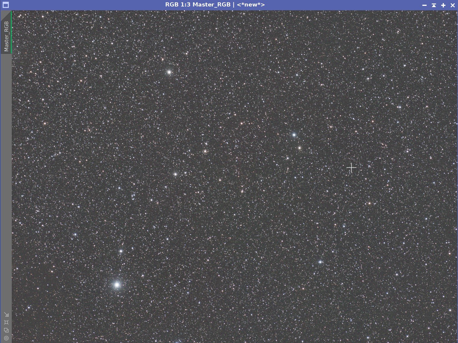
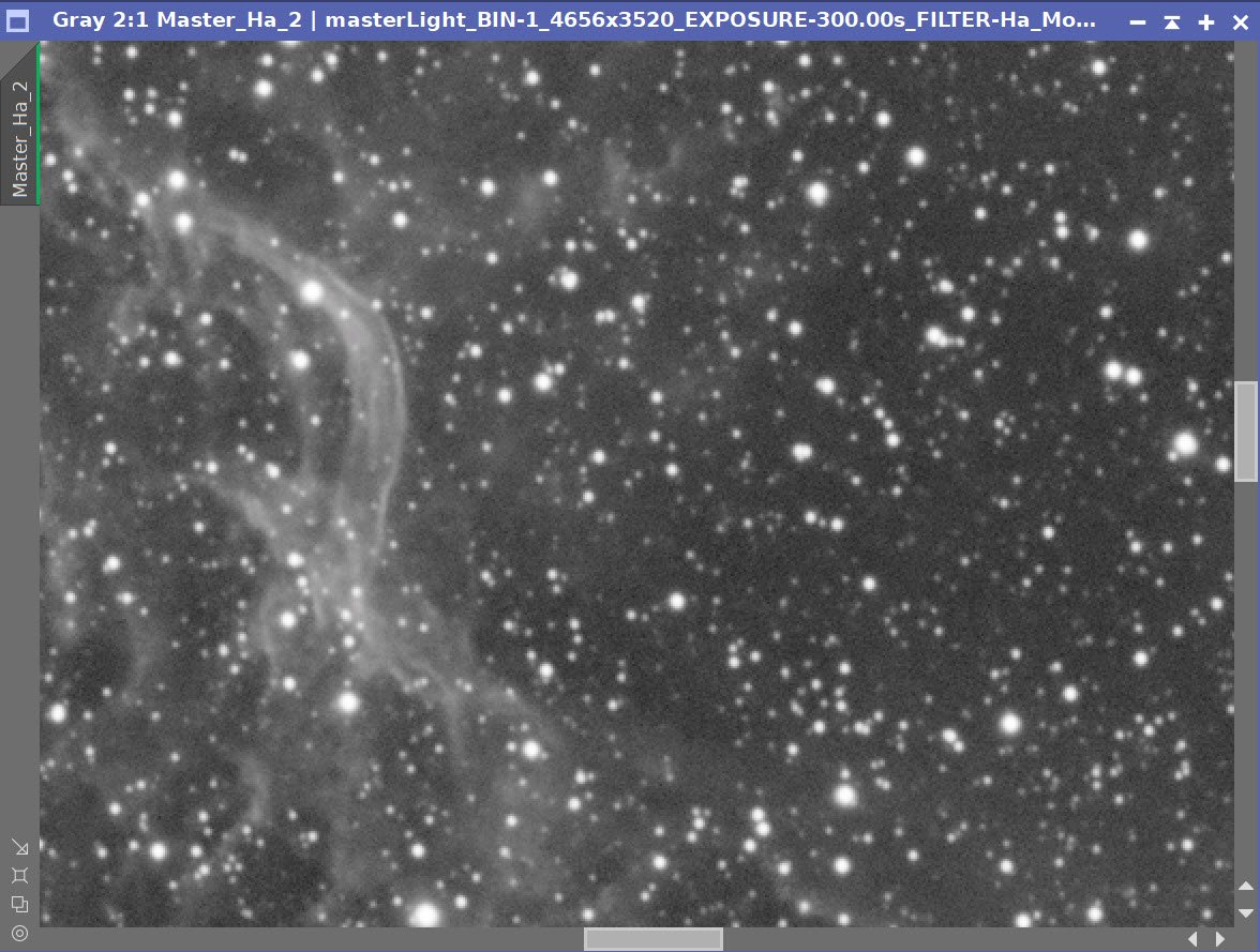
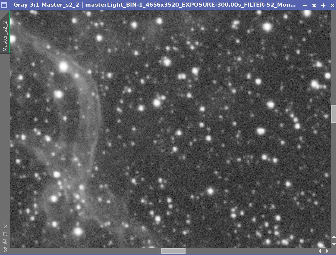
After preprocessing, I ended up with Master Linear images that look like this:

Master Ha is on the right, and Master S2 is on the left. Still a pretty weak signal!
I was beginning to appreciate what a faint target this really was! Here was the single longest integration time I have achieved to date - taken on my fastest scope - and I can just begin to see the signal.
Image Processing Approach
To make this image work, I thought a few key approaches were critical:
The color image would have to be HSS - a variation on the HOO bi-color approach
I would create and use a synthetic luminance image to maximize detail and sharpness
Processing would have to focus on the use of starless images. Otherwise, the extensive stretching of this image would create stars that would be bloated and out of control.
I would then add my RGB stars to give the sky a more natural look.
This is the approach I took, and I think it worked out well. But while some images seem easy to process - this was not one of those images.! To get what I wanted, I needed to be pushing hard, stretching the data - and this made the processing a bit of a challenge.
Discussion of Results
I am much happier with my final result. Having said that, this object is so faint that I think it requires even more integration time. But here, we start to run into diminishing returns.
To double the quality, I need to quadruple the integration! The kind of integration I need here is beyond the means of my local weather patterns and tree line limitations. I am glad I increased the integration, and I am reasonably happy with the result - but I have to conclude that getting the quality I ultimately would like for this target is probably beyond my means!
A detailed Processing Walk-Through is provided for this image at the end of the posting…
Capture Details
Lights Frames
Data was collected over eight nights: July 28, July 30, July 31, Aug 1, Aug 3, Aug 28, Sept 1, and Sept 2.
116 X 300 seconds, bin 1x1 @ -15C, Unity Gain, Astronomiks 6nm Ha
80 X 120 seconds, bin 1x1, @ -15C, Unity Gain, Astronomiks 6nm S2
13 X 90 seconds, bin 1x1, @ -15C, Unity Gain, ZWO Red
10 X 90 seconds, bin 1x1, @ -15C, Unity Gain, ZWO Green
22 X 90 seconds, bin 1x1, @ -15C, Unity Gain, ZWO Blue
Total of 17 hours 27 minutes 30 seconds
Cal Frames
25 Darks at 300 seconds, bin 1x1, -15C, unity gain
25 Darks at 90 seconds, bin 1x1, -15C, unity gain
12 Flats at bin 1x1, -15C, Unity gain - for Ha, S2, R,G,B filters
25 Dark Flats at Flat exposure times, bin 1x1, -15C, gain unity
Software
Capture Software: PHD2 Guider, Sequence Generator Pro controller
Image Processing: Pixinsight, Photoshop - assisted by Coffee, extensive processing indecision and second-guessing, editor regret, and much swearing…..
Capture Hardware:
Scope: Askar FRA400 f/5. 6 Astrograph
Focus Motor: ZWO EAF 5V
Guide Scope: William Optics 50mm guide scope
Guide Scope Rings: Wiliam Optics 50mm slide-base Clamping
Ring Set
Mount: IOptron CEM 26
Tripod: Ioptron 1.5” Tripod
Camera: ZWO ASI1600MM-Pro
Filter Wheel: ZWO EFW 1.2 5x8
Filters: ZWO 1.25” LRGB Gen II, Astronomiks 6mm Ha, OIII,SII
Camera Rotator: Pegasus Astro Falcon
Guide Camera: ZWO ASI290MM-Mini
Dew Strips: Dew-Not Heater strips for Main and Guide
Scopes
Power Dist: Pegasus Astro Powerbox Advanced
USB Dist: Pegasus Astro Powerbox Advanced
Polar Alignment Cam Iplolar
Software:
Capture Software: PHD2 Guider, Sequence Generator Pro controller
Image Processing: Pixinsight, Photoshop - assisted by Coffee, extensive processing indecision and second-guessing, editor regret and much swearing…..
Click below to see the Telescope Platform version used for this image
Image Processing Walk-Through
(All Processing done in Pixinsight - with some final touches done in Photoshop)
1. Blink Screening Process
Ha
Five subs removed for elongated stars. These were caused by a problem in PHD2 guide parameters and this was corrected.
Some very slight cloud gradients - none removed for this
S2
One sub removed due to clouds
Six removed due to elongated stars - see note on PHD2 issue above
Some very slight cloud gradients - none removed for this
Red
Rolling thin clouds - gradients - none removed for this
Elongated stars - Removed two that were the worse.
Green
Minimal gradients
Some trails
Blue
Some trails
Flats
Collected for five of the eight nights. Data looks good
Dark flats
Collected for the first night - data looks good
Darks
Get Darks from the 7-26-22 cal files.
2. WBPP 2.4.5
Reset everything
Load all lights
Load all flats
Load all darks - Darks 90 and 300 from fpa400 6-27-22
Add the “Night” keyword
Select - maximum quality
Registration reference - auto - the default
Select output directory
Enable CC for all light frames
Pedestal value - auto for Ha and S2 frames
Disable drizzle processing
Darks -set exposure tolerance to 0
Map flats and darks across nights
Decided to allow WBPP to do integration
Ran with no problems in 50 minutes.


Post Calibration View.
Note: I was not worried about sharpness in this image, and since I would be removing the stars, I decided NOT to do my normal SubFrameSelector analysis.
Rejection High - Ha (click to enlarge)

Rejection High - Red: (click to enlarge)

Rejection High - Blue: (click to enlarge)
Rejection High - S2 (click to enlarge)
Rejection High - Green: (click to enlarge)
3. Crop all of the images
Load all master images
A common crop level was selected, and DynamicCrop was used to trim all of the master frames.
4. Dynamic Background Extraction
DBE was run for each image using the subtraction method. Below are the Sampling plans, the before image, the after image, and the removed background images.
DBE: Ha Sampling (Click to enlarge)
DBE: S2 Sampling (Click to enlarge)
Ha image Before DBE (click to enlarge)
S2 image Before DBE (click to enlarge)
Ha image After DBE (click to enlarge)
S2 image After DBE (click to enlarge)
Ha background removed (click to enlarge)
S2 background removed (click to enlarge)
DBE: Red Image Sampling (Click to enlarge)
Red Image Before DBE (click to enlarge)
Red Image After DBE (click to enlarge)
Red background removed (click to enlarge)
DBE: Green Sampling (Click to enlarge)
Green image Before DBE (click to enlarge)
Green Image After DBE (click to enlarge)
Green background removed (click to enlarge)
DBE: Blue Sampling (Click to enlarge)
Blue image Before DBE (click to enlarge)
Blue Image After DBE (click to enlarge)
Blue background removed (click to enlarge)
5. Create and Process the Linear RGB Color Star Images
Create an initial RGB image by running ChannelCombination
Run PCC
Running Noise XTerminator with a value of 0.5 in linear mode
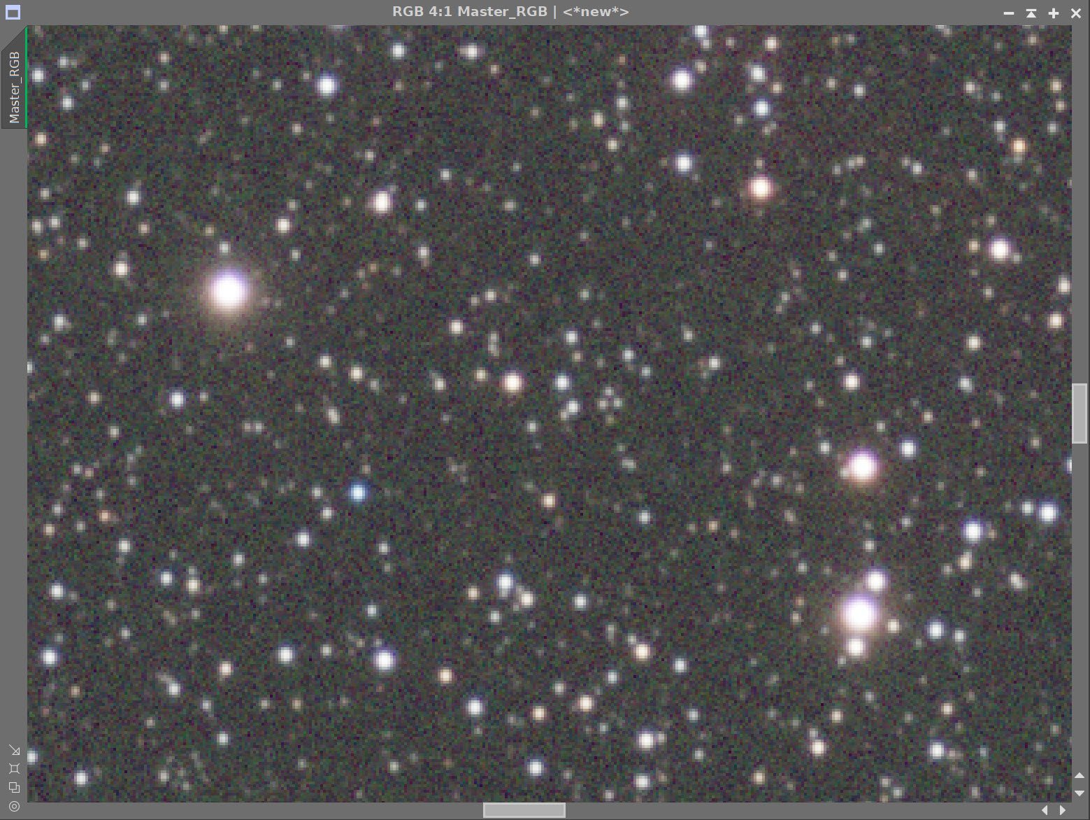
Initial Master RGB Star Images (click to enlarge)

PCC Regression Line
Master_RGB Star image after PCC.
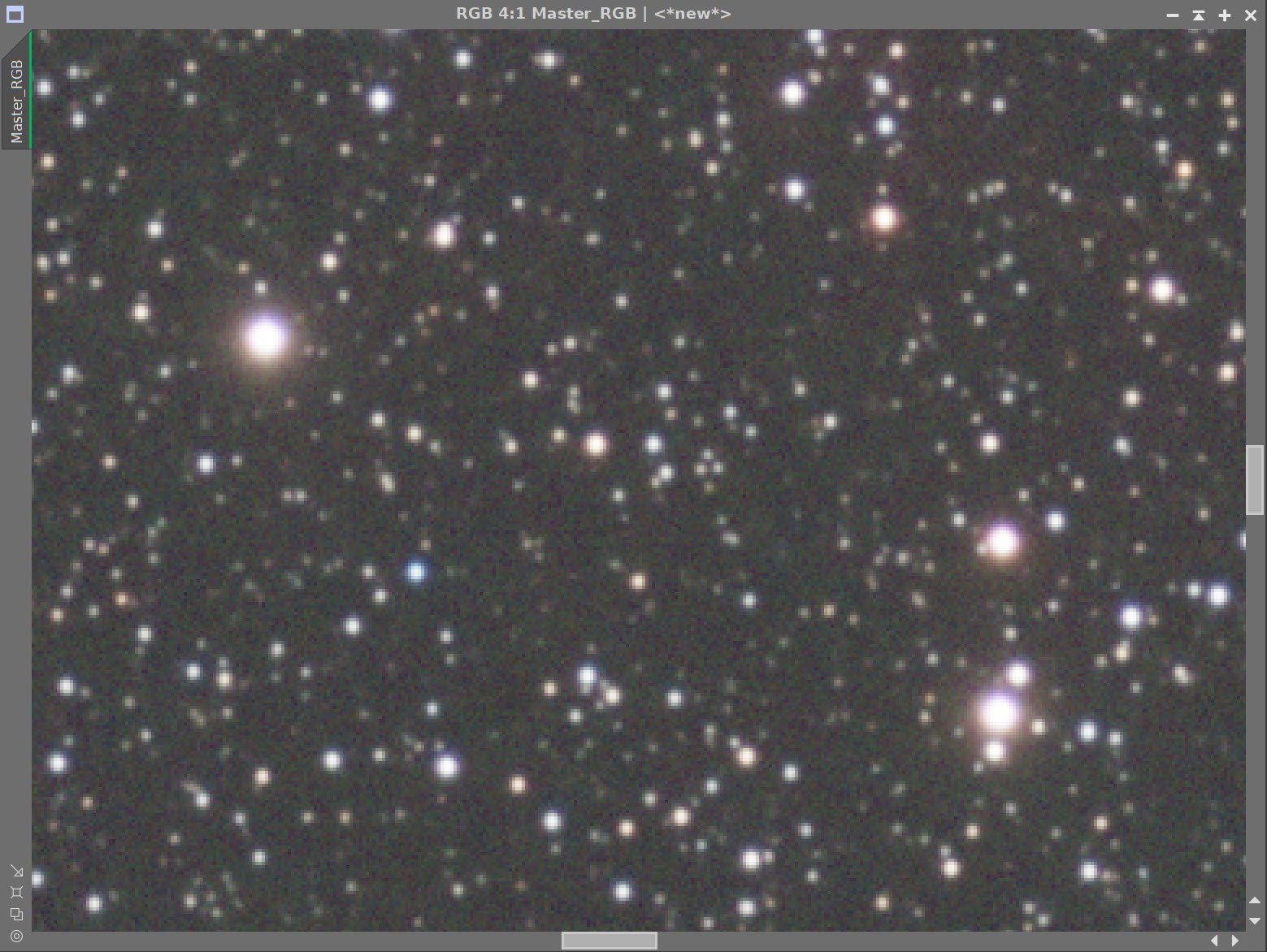
Before and After application of RC Noise XTerminator with a value of 0.5
6. Create the Synthetic Luminance Image and Process
Using PixelMath, create a new Luminance image by using this expression:
(0.75 * Master_Ha)+(0.25 * Master_S2)
Prep for deconvolution
Run PFSImage and create the pfs image
Run StarMask to create the initial LDSI image. (see StarMask settings below in the panel screenshot)
Use HT (see panel screenshot below for curve uses) to boost the LDSI mask.
Select multiple Previews of the Ha image for Decon parameter exploration.
Iteratively test deconvolution with various parameters until the best result is obtained.
Run Deconvolution on the Master_L image
Note: There was relatively little gain seen from this deconvolution effort. The FRA400 scope is slightly under-sampled, and I find that decon really wants well-sampled or over-sampled stars. If I had Drizzled Processed this image, I would have likely seen more impact. The synthetic nature of the L image may also play a role here.
Run Noise XTerminator in linear mode with a value of 0.5

Master L - a synthetic combination of 75% Ha and 25% S2

PFSImage Panel after PSF has been computed for L

PFS Image

StarMask settings used to create the LDSI mask.

HT boost settings for the LDSI mask

The final LDSI image for L

Preview areas selected for Deconvolution parameter testing.

Final Decon Values used for Synthetic L

Linear Ha Image Before and After Decon, and After Noise XTerminator 0.5
7. Create the Color HSS Image
Apply Noise XTerminator with a value of 0.5 with linear mode checked - for both the Maser Ha and S2 images
Use the AIP-SHO Script to explore ways of creating the HSS image. The final one chosen was:
Red: 100% Ha
Green: 100% S2
Blue: 85% S2 and 15% Ha


Ha and S2 Images: Before and After Noise XTerminator 0.5


Master HSS Blended image
8. Take Images Nonlinear
Take the L image Nonlinear
Select a preview area on a good sample of the background sky.
Run MaskedStretch with the preview above
Tweak with CT
Take the HSS image Nonlinear
Select a preview area on a good sample of the background sky.
Run MaskedStretch with the preview above
Tweak with CT
Take the RGB Star image Nonlinear
Select a preview area on a good sample of the background sky.
Run MaskedStretch preview above
Tweak with CT
L image after MaskedStretch (click to enlarge)
HSS image after MaskedStretch (click to enlarge)
RGB Star image after MaskedStretch (click to enlarge)
L after initial CT to adjust tone scale (click to enlarge)
L after initial CT to adjust tone scale (click to enlarge)
L after initial CT to adjust tone scale (click to enlarge)
9. Create Starless Versions of L and HSS images
Make a copy of the nonlinear L and HSS images.
Run Starnet2 on each.
L and HSS Starless image
10. Create Stars Only RGB Image
Make a copy of the nonlinear RGB Stars Image
Run Starnet2 to create a starless version
Run PixelMath and subtract the starless version from the original.

RGB Stars only
11. Integrare L starless Image into the HSS Starless Image
LRGBCombnation will cause the image to lighten, and the reds will start to go pink. In preparation for this, use CT to darken both the L and HSS Starless images
Use LRGBCombination to fold the L starless image into the HSS starless image.
Adjust final image with CT
Darkened L starless image (click to enlarge)
Darkened HSS Starless Image (click to enlarge)
HSS after L insertion (click to enlarge)
After a CT application to make things a bit snappier (click to enlarge)
12. Add Stars Back into the Image
Use PixelMath to add the current HSS image and RGB Stars Image back together
The final image is still too pink in color - we will deal with that later.

RGB Stars added.
13. Do Star Reduction
Use Bill Blanshan’s Star Reduction Method:
Create Starless image for the reduction using Starnet2
Apply method 2 with a value of 0.35
Blanshan SR Icons

Starless image for use with Blanshan SR
Before Star Reduction (click to enlarge)
After Star Reduction (click to enlarge)
14. Do final Image Processing
Rotate the image 90 degrees counterclockwise so that the “Dragon” Seems right-side up.
Deal with the “Pink” color:
Create a mask with the ColorMask script for red tones.
Apply the red mask to the HSS image
Use CT to adjust the Red curve and the saturation to make the nebula less pink and redder.
Remove the mask
Apply Noise XTerminator with a value of 0.6
Sharpen the image with MLT (see screen snap below for settings used)
FInalize the Crop

After 90 degree rotation

Red Mask

Red Mask Applied, CT adjustment with Red Curve and Saturation to deepen red tones.
The Final Crop

MLT Panel showing the sharpening parameters used.

Before and After final Noise XTerminator Application, and with Sharpening
15. Export to Photoshop
Save image as Tiff 16-bit unsigned and move to Photoshop
Use Raw Camera Filter to adjust Global Clarity, Texture, and Color Mix
Use a lasso with a 150-pixel feather to select smaller areas of nebulosity and enhance wit Clarity slider, color mix, and red luminance adjustments,
Use StarShrink to reduce just the largest stars further.
Add watermarks
Export Clear, Watermarked, and Web-sized jpegs.
And the final image…
After doing manual camera rotations to achieve the compositional framing that I plan - using SGP’s Framing and Mosaic Wizard - I finally decided to add a Camera Rotator to this rig to automate the rotation between objects and when getting flat cal frames for images shot with a specific camera rotation. While I had the rig apart, I re-tensioned the declination belt on the mount to reduce declination backlash.