
NGC 6979: Pickering’s Triangle ~ 12 hours in SHO
Date: Sept 11, 2022
Cosgrove’s Cosmos Catalog ➤#0111
Updates:
09-11-22: Added a section discussing the surprising personality differences between color filter images
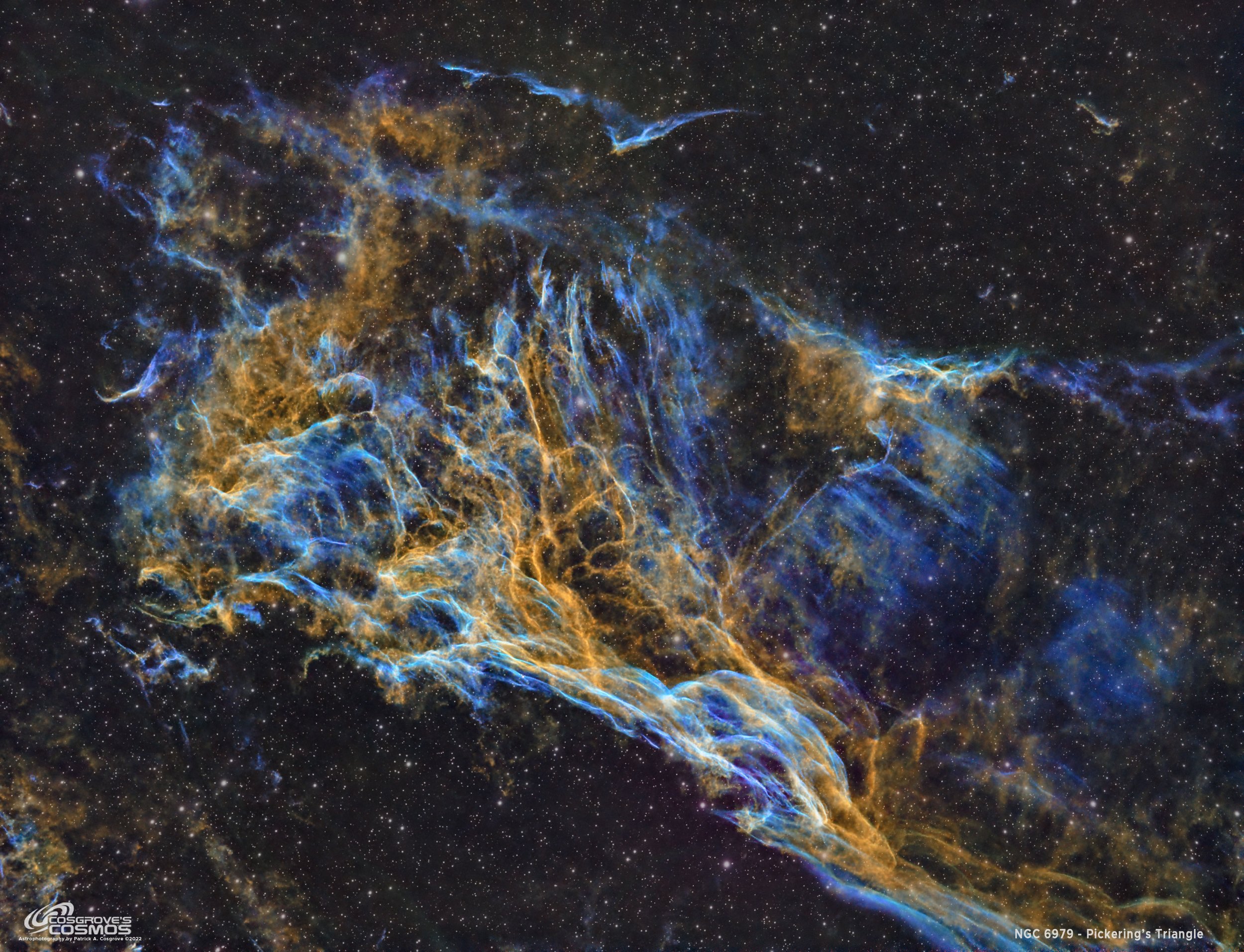
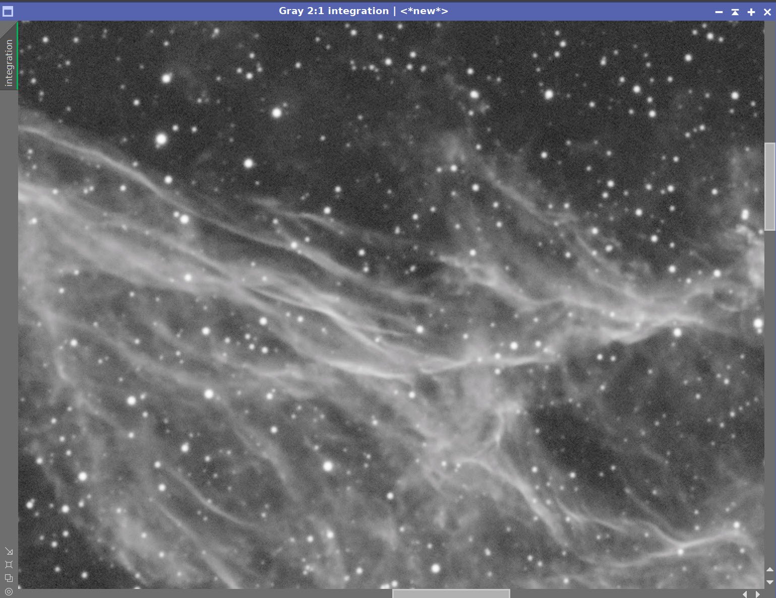
Pickering’s Triangle is a smaller, dimmer portion of the impressive Cygnus Loop and Veil Nebula in Cygnus. (click on the image for full res version via Astrobin.com)
Table of Contents Show (Click on lines to navigate)
About the Target
Pickering’s Triangle, also known as Pickering’s Triangular Wisp, is a smaller and dimmer portion of the larger Cygnus Loop or Veil Nebula.

Screen snap of Stellarium, showing the Cygnus loop in its entirety. I have marked where Pickering’s Triangle can be found.
It was discovered via photograph by Williamina Fleming in 1904, but the credit went to the director of the observatory, Edward Charles Pickering.
Interesting side note: Williamina Fleming originally worked as a maid to Pickering, the director of the Harvard College Observatory. He saw something in her and hired her to do administrative work at the observatory. He eventually taught her how to analyze stellar spectra, and she became the founding member of the all-women group of “Human Computers” that supported data analysis for projects done by the observatory!

Williamina Fleming (1857-1911) Image from Wikipedia
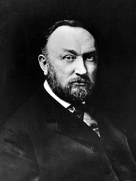
Edward Charles Pickering (1846-1919) image taken from Wikipedia.
Since this was discovered after the New General Catalog was published, it has no formal NGC designation. NGC 6979 is commonly referenced for this object, but this is technically incorrect.
The Veil Nebula is a remnant of a supernova. Wikipedia summarizes it like this:
The source supernova was a star 20 times more massive than the Sun, which exploded between 10,000 and 20,000 years ago. At the time of explosion, the supernova would have appeared brighter than Venus in the sky, and visible in daytime. The remnants have since expanded to cover an area of the sky roughly 3 degrees in diameter (about 6 times the diameter, and 36 times the area, of the full Moon). While previous distance estimates have ranged from 1200 to 5800 light-years, a recent determination of 2400 light-years is based on direct astrometric measurements. (The distance estimates affect also the estimates of size and age.)
The Triangle itself is a very complex network of shimmering filaments and expanding gas clouds that can be a feast for the eyes. The area is rich in molecular glasses and shines in the light of excited Hydrogen, Oxygen and Sulfur.
The Annotated Image

Very little annotation for this image, as it was discovered after the NGC was published! This annotated image was created in Pixinsight, using the ImageSolver and Annotate Image Scripts.
The Location in the Sky

This finger chart was created in Pixinsight using the FinderChart process.
About the Project
Introduction
A few minutes of introduction for this project by yours truly! Yet another video was created. I thought this was supposed to improve with practice! I thought this would get easier to do! Neither seems to be the case so far - but I will stick with it. After all, I am not sure it can get worse, so there is only one way to go!
Please consider subscribing to my fledgling Youtube Channel and RIng the bell. I could use the support to get this off the ground! Thank you!
Choosing the Target
During the last imaging session, Cygnus was still well positioned, and when choosing targets, I combed over the objects that could be found there. Recently, I shot the Bat Nebula (NGC6995), a zoomed-in study of a portion of the Cygnus Loop.
I considered doing something like that again.
In the past, I have heard about a portion of the Cygnus Loop called Pickering’s Triangle. While I have heard the name, I was unfamiliar with it.
After some digging, I found some information on it, but the fact that it did seem to have a formal NGC designation made it kind of an oddball. But I was able to find information about it by searching for its popular name and I found a treasure trove of wonderful images of it on Astrobin.com. Like the Bat Nebula, this was a very complex section of sky, with many shimmering and overlapping filaments and sheets of nebulosity.
Interestingly, almost every image of Pickering’s Triangle that I saw was a bi-color image in the HOO palette. I knew from experience that the Bat Nebula had a pretty strong signal in all three primary narrowband channels, so I thought I would do my own take on it using the SHO palette.
I used my William Optics 132mm platform and was able to use SGP’s Framing and Mosaic Wizard to set up the composition. This was a little tricky since it did not have its own designation that I could search by, and the search function on the Framing and Mosaic Wizard could not find anything using its common name. So I search for other objects in the neighborhood and scrolled over to the triangle for framing and composition.
Data Capture
I captured 5-minute subs over four nights: Aug 24, Aug 28, Sept 1, and Sept 2. In general, these nights were clear and cool. The first night was cut short when some high-level clouds rolled in after an hour of shooting. The rest of the nights were excellent.
Data Analysis
Blink analysis showed that the data looked pretty good in general. A total of 11 5-minute subs were removed due to clouds coverage. That was a lost hour. In addition, SubFrameSelector Analysis for FWHM and Eccentricity eliminated another 1.25 hours. So I lost about two hours of data from all of the subs collected - a loss rate of about 14%. In the past, I would have just used them all and hoped that integration statistics and rejection algorithms would make up for the difference. And to an extent, I think it does. But I have also found that my images are much sharper when I remove the ones that have star growth and eccentricity problems.
I also had to eliminate a few subs because the images had bad data! What I mean is that the digital image of the sub showed some strange electronic interference pattern. This occasionally happens with this camera, and I do not know why.

Example of an abnormal sub that sometimes is produced by mu ASI1600MM-Pro camera. My other ASI1600MM-Pro camera does not produce these ever…
Fascinating Filter Personalities
As I process these narrowband images, I work my way through the linear operations, and then I take the images non-linear. At this point, I often stop and take a careful look at these nonlinear master images before I begin to combine them and move on.
The three images always have some differences, or else the color images you form would pretty dull and boring. So differences are expected.
But with some objects, those differences are so dramatic that it is almost like you were imaging very different targets!
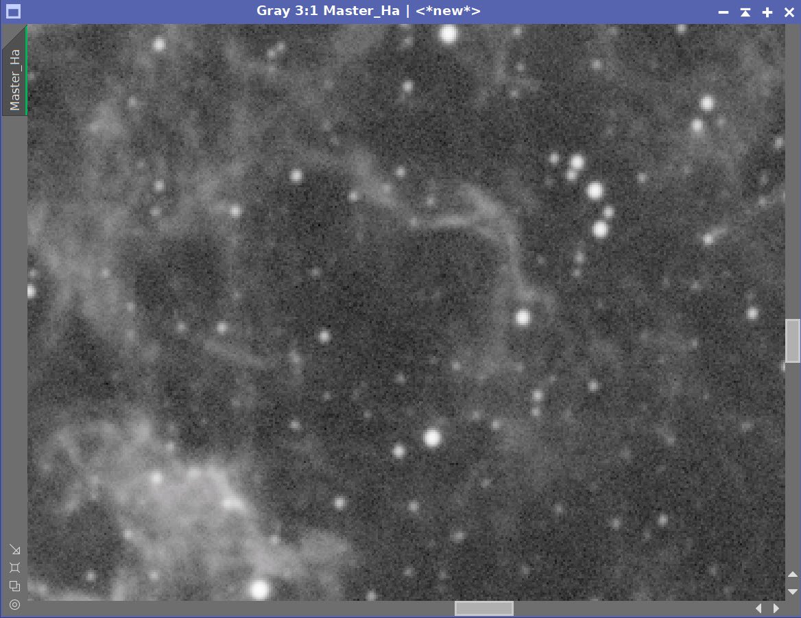
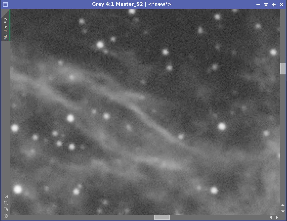
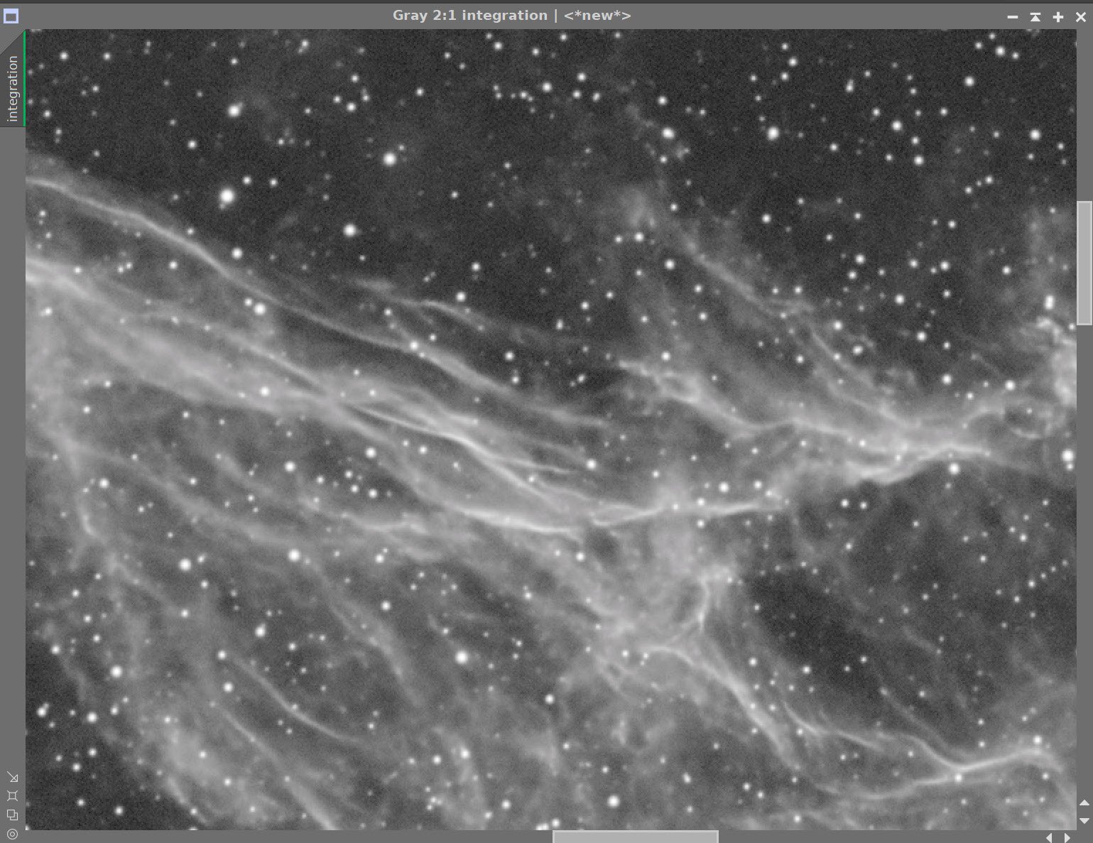
Pickering’s Triangle is one of those objects. The Ha and the S2 image has some strong structural similaries as can be seen here:
The Ha Nonlinear Image
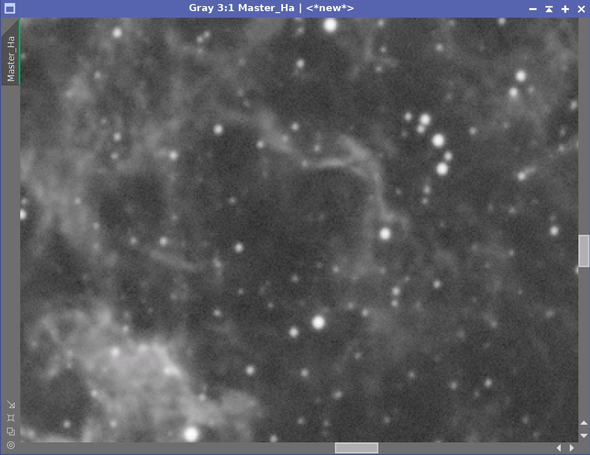
The S2 Nonlinear Image
These images have a rough, almost jaggedy type of structure.
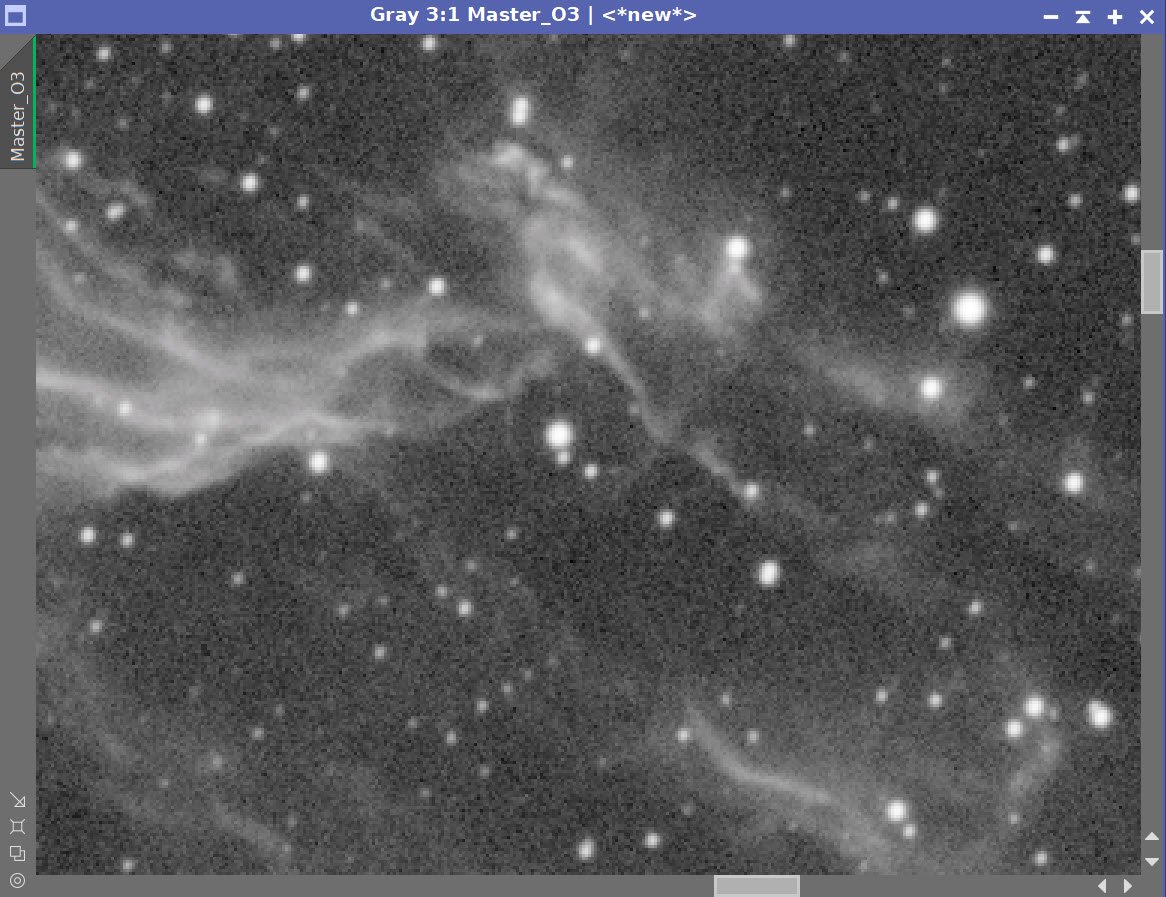
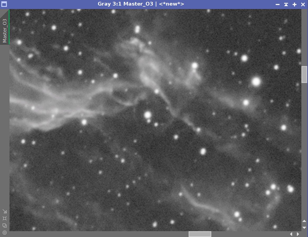
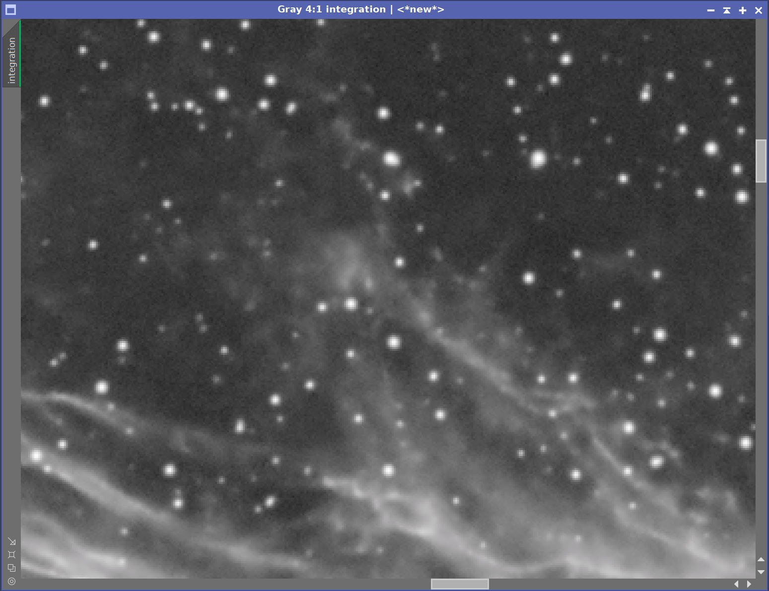
Now let’s compare those with the O3 nonlinear Image:
The O3 nonlinear Image
What an amazing difference. Smooth and silky! Long flowing wisps of smoke. Subtle sheets with graceful folds and twists. It’s really quite beautiful!
I am fascinated by these differences.
I have seen huge differences in my narrowband image of M27 as well.
What other objects have you seen that have these kinds of differences?
Previous Efforts
While I have never shot Pickering’s Triangle before, I have shot various sections of the Cygnus loop. Those images are seen below - click on them to go to the postings for those images.
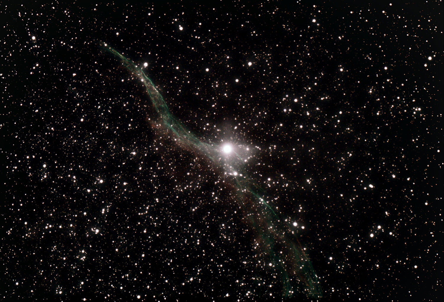
NGC 6960 - The Witches Broom - Aug 2019
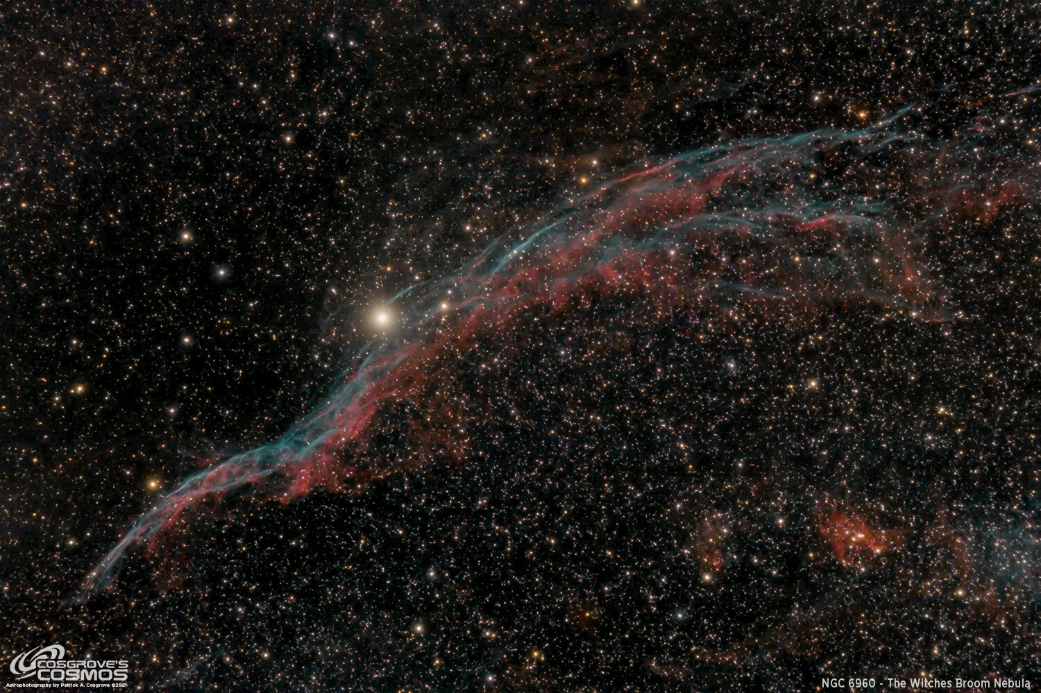
NGC 6960 - The Witches Broom - July 2020
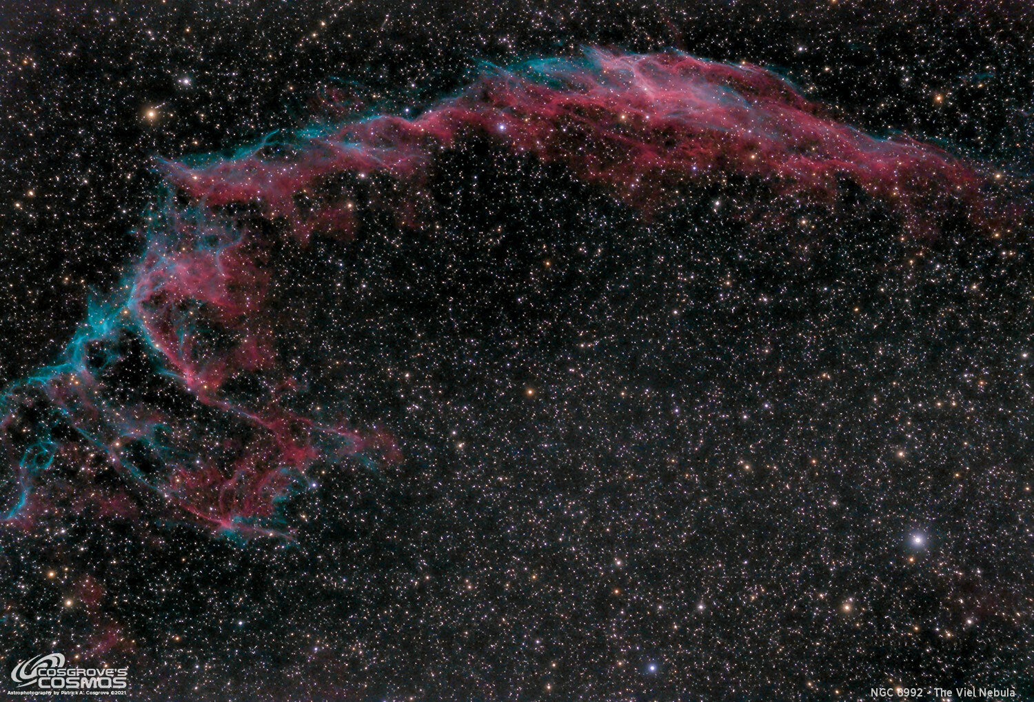
NGC 6992 - The Veil Nebula - July 2020
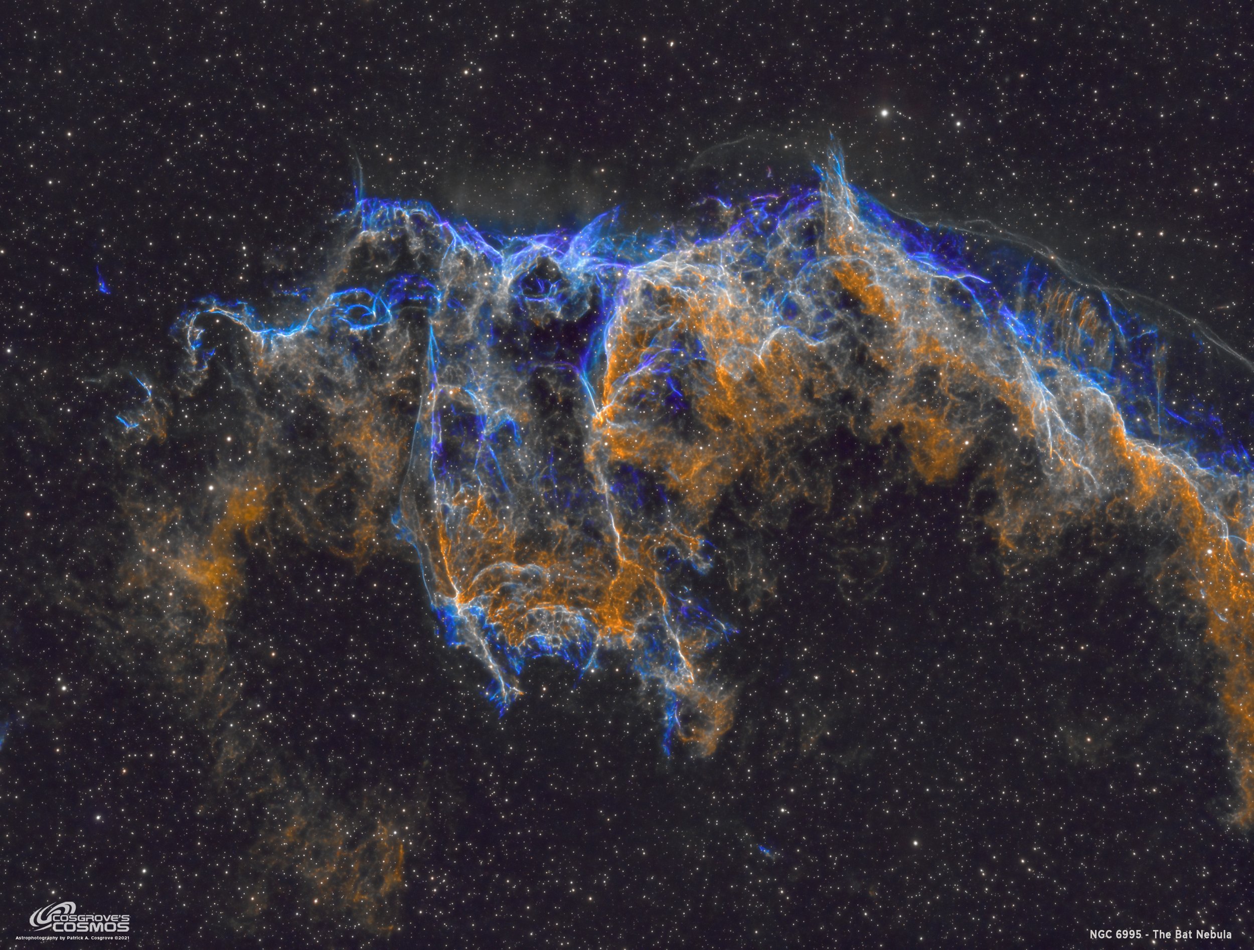
NGC 6995 - The Bat Nebula - Aug 2022
Image Processing
Image processing was pretty straightforward. I created a synthetic luminance image by using ImageIntegration to combine the three master images, and this L image was then used for deconvolution and general image sharpness and detail, while the others contributed color info.
Early in the process I shifted over to starless and starred image processing worklows - this allowed me to aggressively stretch the nebulae without impacting the stars.
This is also the first image where I used the Color Mask Generation tools created by Bill Blandshan. These seem to work very well.

Bill Blanshan’s Color Mask Icons
It is also the first time that I used the StarBlend script written by James Lamb. This also worked very well for me!

James Lamb’s Star Blend script
A detailed Processing Walk-Through is provided for this image at the end of the posting…
More Information
Wikipedia: The Veil Nebula
Sky & Telescope: Pickering’s Triangle
APOD.Nasa.Gov: Pickering’s Triangle
Capture Details
Lights Frames
Data was collected over four nights: Aug 24, Aug 28, Sept 1, and Sept 2
Number of subs after Blink and SubFrameSelector analysis and removal
64 x 300 seconds, bin 1x1 @ -15C, Gain Zero, Astrodon 5nm Ha
45 x 300 seconds, bin 1x1 @ -15C, Gain Zero, Astrodon 5nm O3,
33 x 300 seconds, bin 1x1 @ -15C, Gain Zero, Astronomiks 6nm S2
Total of 11.83 hours
Cal Frames
25 Darks at 300 seconds, bin 1x1, -15C, gain Zero
12 Flats at bin 1x1, -15C, gain Zero - for Ha, R, G & ,B filters
25 Dark Flats at Flat exposure times, bin 1x1, -15C, gain unity
Software
Capture Software: PHD2 Guider, Sequence Generator Pro controller
Image Processing: Pixinsight, Photoshop - assisted by Coffee, extensive processing indecision and second-guessing, editor regret, and much swearing…..
Capture Hardware:
Scope: William Optics 132mm f/7 FLT APO Refractor
Focus Motor: Pegasus Astro Focus Cube 2
Cam Rotator: Pegasus Astro Falcon
Guide Scope: Sharpstar 61EDPHII
Guide Focus Motor: ZWO EAF
Mount: Ioptron CEM 60
Tripod: Ioptron Tri-Pier
Camera: ZWO ASI1600MM-Pro - new
Filter Wheel: ZWO EFW 1.2 5 x8 - new
Filters: ZWO Gen II 1.25” LRGB,
Astrodon 5nm Ha,
Astrodon 5nm Ha,
Astronomiks 6nm S2
Guide Camera: ZWO ASI290MM-Mini
Dew Strips: Dew-Not Heater strips for Main and Guide Scopes
Power Dist: Pegasus Astro Pocket Powerbox
USB Dist: Startech 8 slot USB 3.0 Hub
Polar Align Cam: Polemaster
Software:
Capture Software: PHD2 Guider, Sequence Generator Pro controller
Image Processing: Pixinsight, Photoshop - assisted by Coffee, extensive processing indecision and second-guessing, editor regret and much swearing…..
Click below to see the Telescope Platform version used for this image
Image Processing Walk-Through
(All Processing done in Pixinsight - with some final touches done in Photoshop)
1. Blink Screening Process
Ha
Five frames were removed- clouds or bad data
O3
Three subs removed for clouds
Some trails
Some slight gradients
S2
Three rejected for clouds or bad data
Some gradients
Flats
Collected for the first night only. Data looks good
Dark flats
Collected for the first night - data looks good
Darks
Get Darks from the 7-26-22 cal files.
2. WBPP 2.5.0
First use of version 2.5.0 - still not yet familiar with its new features.
Reset everything
Load all lights
Load all flats
Load all darks - 300 sec from 7-26-22 cal data
Add the “Night” keyword
Select - maximum quality
Reg reference - auto - the default
Select output directory
Enable CC for all light frames
Pedastal value - auto for filters
Darks -set exposure tolerance to 0
Deselect integration mode - just cal and alignment
Map flats and darks across nights
Ran with no problems - 55 minutes

WBPP Calibration view.

Post Calibration View.
3.0 Use SubFrameSelector to analyze the Calibrated subs
After WBPP ran, I used SubFrameSelector to check the quality of my subs.
Subs for each filter were loaded into the tool, and metrics were computed. FWHM and Eccentricity were the key metrics I used in this analysis. Screenshots for each filter are attached below.
Ha images: 6 deleted: 1 for having too high an FWHM and 5 for Eccentricity value
O3 images: 6 deleted: 5 for having too high an FWHM and 1 for Eccentricity value
S2 images: 3 deleted: 1 for having too high an FWHM, and 2 for Eccentricity value
This lost me 1.25 hours of subs.
Ha Sub FWHM - Note eliminated frames (click to enlarge)
O3 Sub FWHM - Note eliminated frames (click to enlarge)
S2 Sub FWHM - Note eliminated frames (click to enlarge)
Ha Sub Eccentricity - Note eliminated frames. (click to enlarge)
O3 Sub Eccentricity - Note eliminated frames (click to enlarge)
S2 Sub Eccentricity - Note eliminated frames (click to enlarge)
4. Integration
ImageIntegration
ImageIntegration was run for each Master image.
The same setup was used for each run.
ESD was chosen for rejection.
Large scale rejection checked - 2x2
A sample panel for ImageIntegration can be seen below

ImageIntegration panel settings.
Very little needed to be rejected here as the images were very clean.
Rejection High - Ha (click to enlarge)
Rejection High - O3: Note trails removed (click to enlarge)

Rejection High - S2: (click to enlarge)

Initial Master Ha, O3, and S2 images!
5. Crop all of the images
A common crop level was selected, and DynamicCrop was used to trim all of the master frames.
The edges were remarkably clean. Only a little had to be removed from the left-most edge.
6. Dynamic Background Extraction
DBE was run for each image using the subtraction method. Below are the Sampling plans, the before image, the after image, and the removed background images.
DBE: Ha Sampling (Click to enlarge)
Ha image Before DBE (click to enlarge)
Ha image After DBE (click to enlarge)
Ha background removed (click to enlarge)
DBE: O3 Image Sampling (Click to enlarge)
O3 Image Before DBE (click to enlarge)
O3 Image After DBE (click to enlarge)
O3 background removed (click to enlarge)
DBE: S2 Sampling (Click to enlarge)
S2 image Before DBE (click to enlarge)
S2 Image After DBE (click to enlarge)
S2 background removed (click to enlarge)
7. Apply light Noise Reduction to Linear Master Images
Apply Noise XTerminator with a value of 0.5 and the linear mode box checked.

Master Linear Ha, O3 & S2 Images - Before and After Noise XTerminator 0.5 Linear.
8. Create and Process the Synthetic Lum image.
Save linear Ha, O3, and S2 images to file, so that ImageIntegration can access them.
Configure ImageIntegration:
Load the three files
Disable rejection
Run ImageIntegration and save the resulting image as Mastere_L
Prep for Deconvoluton
Run PFSImage script and computer the PSF file
Run StarMask (see panel snap for parameters)
Use HT (configured as shown in screen snap) to boost mao
Rename LDSI
Select some Preview regions for decon parameter testings.
Iteratively test parameters until best results are obtained (see screen snap below for final values)
Apply decon to Master_L image
Apply Noise XTerminator with a value of 0.45 in linear mode.

This is the set up I used to create the Synthetic Luminance image

Here are the weights reported by ImageIntegration. O3 seemed to be the dominant image in this group.

The Computed Luminance image. I find this image to be quite beautiful on its own!

The PSFImage Script Panel after it has computed the PSF.

The PSF image ( the cross is a screen capture “oops”).

Here is the set up I used to create the LDSI Star Mask.

Boost used to enhance the LDSI image.

The Final Local Deringing Support Image (or LDSI)

These final values were determined by iterative testing.
Before and After application of Deconvolution

Master_L: Before and After Noise XTerminator - value 0.5 linear
9. Create Initial Nonlinear SHO Image
Go nonlinear with all images
Use the STF->NT Method
This is simple and keeps the main relationships between colors the same. The only problem is that stars grow, but we will deal with that differently later on!
Use HT to remove dead space located left of the histogram
Apply LHE with a radius of 64, a contrast limit of 2.0, an amount of 0.1, and a histogram of 8-bits.
Create a color image
Use LRGBCombination and add nonlin S2, Ha, O3, and L for the neutral
Other parameters all at default values.
Run - creating first color SHO image.
Nonlinear Ha Image (click to enlarge)
Nonlinear O3 Image (click to enlarge)
Nonlinear S2 Image (click to enlarge)
Nonlinear L Image (click to enlarge)

The initial Nonlinear SHO image!
10. Process the SHO Color Image
Rotate the Image 180 degrees for a better composition
Apply SCNR for green at 80%
The SHO image rotated 180 degrees - I think this works better for composition. (click to enlarge)
After SCNR is applied to get 8% of the Green out. (click to enlarge)
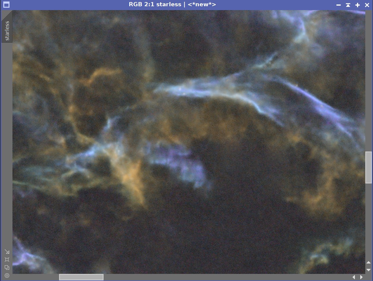
Create and process Starless Images:
Copy the image and name it “starless”
Apply Starnet 2 to it.

The initial Starless image.
Apply Noise XTerminator with a value of 0.65
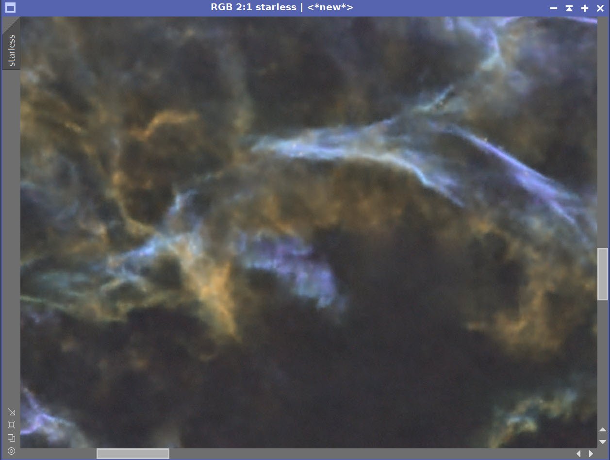
Before and After Noise XTerminator with value of 0.65
Apply CT to the whole image and adjust tone and color

Global CT adjustment for color and sat.
Create Blue Mask with Bill Blnshand script for BlueMask, one blur cycle
Create a Yellow mask with above - one blur cycle
Use CT to boost the masks a bit
Blue Mask (click to enlarge)
Yellow Mask (Click to enlarge)
Apply blue mask, adjust with CT
Apply yellow mask, adjust with CT
Blue Mask Adjust (click to enlarge)
Yellow Mask Adjust (click to enlarge)
Create “Stars” Image
Using the original SHO image, use Starnet2 to create a new star mask - name it “stars”
CT to reduce brightness just a bit
Initial Star Image (click to enlarge)
Slightly darkened Star Image (click to enlarge)
Add stars back in using James Lamb’s Starblend script:

Here is the str blending script used.
The Stars are now added back in! (click to enlarge)
Make a copy of this newly starred image and name it SHO_Final
Make a new starless image for use with Bill Blansan’s Str Reduction Method
Use Bill Blansshand SR Method #1 with a value of 0.35
Before Star Reduction (click to enlarge)
After Star Reduction (click to enlarge)
The Background is a little magenta - let’s fix that!
Create a range mask of the background sections
Apply the mask and use CT to reduce magenta saturation

Range Mask for isolating background
Using the range mask, the magenta is removed (click to enlarge)
Apply LHE with A radius of 122, a contrast limit of 2.0, an amount 0.15, and 12-bit histograms

Final SHO image with LSE applied
11. Export to Photoshop
Save images as Tiff 16-bit unsigned and move to Photoshop
Use Camera Raw Filter to adjust Global Clarity, Texture, and Color Mix
ColorMix is much easier to use to adjust hues in an image compared to the tool provided by Pixinsight, and I tend to do this final operation in PhotoShop
Use StarShrink to reduce just the largest stars further. Add watermarks
Export Clear, Watermarked, and Web-sized jpegs.
Our final image!
I was very excited to get the ZWO ASI2600MM-Pro camera a while back. I ordered it when it was announced and then prepared to wait a long time to get it. When I did get it - I decided to put it onto the AP130 platform. That meant that I could move the ZWO ASI1600MM-Pro, along with its filter wheel over to my William Optics Platform. This now means that all of the platforms have been moved over to a mono camera and my ZWOASI924MC-Pro is now not in use.