
Messier 27 - The Dumbbell Nebula in Narrowband - 10.25 Hours
Date: Sept 15, 2021
Cosgrove’s Cosmos Catalog ➤#0084
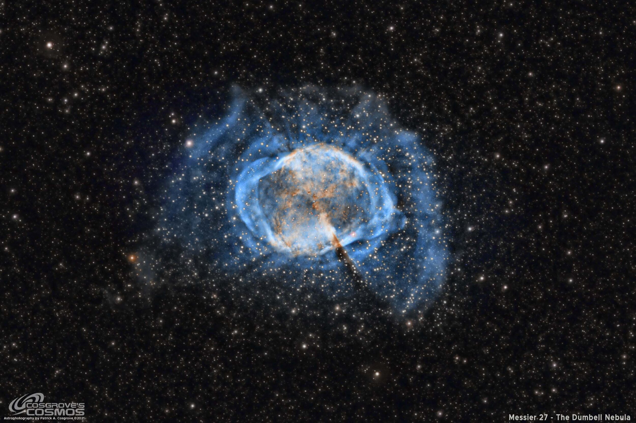
Messier 27 - The Dumbbell Nebula rendered in the Hubble Palette (click on image for full resolution via Astrobin.com)
Published in the May 2022 Issue of Astronomy Magazine!
This image was highlighted in the reader’s Gallery Section with an excellent little summary of the image. This is the third image I published so far in 2022!
Thanks, Astronomy Magazine!

The May 2022 issue of Astronomy Magazine

My image of M27!
Published in Amateur Astrophotography Magazine!
April 9th, 2023 - In issue #111, p70-75. This image was published as part of a profile article on me!


Table of Contents Show (Click on lines to navigate)
A Special Note:
At a later date, I ended up reprocessing this image in May 2023 using new tools and techniques, creating what I believe to be a superior image. This can be seen HERE.

The Improved image. (click to go to the newer post)
About the Target
Messier 27, also known as NGC 6853, the "Dumbell Nebula", and the "Apple Core Nebula" is a planetary nebula located about 1200 light-years away in the constellation of Vulpecula. It was the first planetary nebula ever discovered by Charles Messier in 1764. Planetary nebulae are formed when stars throw off their outer layers of gas as they reach the end of their lives. Based on studies made on its expansion rate, we can work backward to determine that the formation of this nebulae began about 10,000 years ago. Being bright and easily observable even with a small scope, M27 is famous and well known.
The basic form of the nebula is an oblate sphere with a dimension of about 8 arc minutes. There is a void on each side of the sphere, causing its characteristic shape. Given its size and inherent brightness, this shape can easily be seen, thus driving its popular names of the Dumbell and the Apple Core Nebula. Early observers debated whether this was a single nebula or two nebulae close together, and some wondered if the nebulosity consisted of unresolved stars. In John Hershels observing logs of 1833, he noted the following:
“h 2060 = M 27.
Sweep 166 (Auguat 17, 1828)
RA 19h 52m 8.6s, NPD 67d 43m +/- (1830.0) [Right Ascension and North Polar Distance]
(See fig 26.) A nebula shaped like a dumb-bell, with the elliptic outline completed by a feeble nebulous light. Position of the axis of symmetry through the centres of the two chief masses = (by microm.) 30.0deg .. 60.0 deg nf..sp. The diam of the elliptic light fills a space nearly equal to that between the wires (7' or 8'). Not resolvable, but I see on it 4 destinct stars 1 = 12 m at the s f edge; 2 = 12.13 m, almost diametrically opposite; 3 = 13 m in the n p quarter, and 1 = 14.15 m near the centre. Place that of the centre. “
He may have been the first person to use the descriptor of a Dumbbell - I don't know this for certain, but I can say that his observing logs were a lot more precise than mine ever were!
The Annotated Image

This annotated version of Messier 27 was created with Pixinsight ImageSolve and AnnotateImage scripts.
The Location in the Sky

IAU/Sky & Telescope Constellation Map for Vulpecula - M27 is indicated with the yellow arrow.
About the Project
We had three clear nights in early September, those being on the 1st, then the 4th, and the 6th. I tried to find an interesting target for my AP130 platform with its newer ASI2600MM-Pro camera. I considered several possibilities but I finally decided on M27.
Target Selection
Why M27? It is certainly bright and well known - making it a pretty common astrophotographic target. When reviewing images of M27 in Astrobin, I found a long list of very similar images - mostly shot in OSC RGB or Mono Camera LRGB. I also noted that extremely few of these images were awarded "Top Pick" or "Image of the Day". I suppose when everybody and their brother is shooting such a target - after a while - it begins to lose its novelty, and the flood of such images makes it hard to notice a good one.
The other thing I noticed was that there were very few narrowband images of this object. I thought it might be interesting to have a go at that.
I have photographed this object twice before - once in 2019 (you can see that post HERE) and again in 2020 (you can see that HERE). Knowing what those looked like, I was curious to see how narrowband would look by comparison.
So I gathered three nights of data for a total of a little over 10 hours. I preprocessed the images and looked at the resulting Master Ha, O3, and S2 images in Pixinsight.
At first, the images seemed washed out and lacking in detail - at least until I started my processing. As I worked on them, I uncovered astonishing structures buried in the bright nebula, which I had never seen on M27 before. Even more interesting, I found that each image had a very different nature.
Image Processing Discussion
In this next section, I will provide an overview of the image processing done for this project. This is high level. However, I keep a processing log for this image, and that will be listed below for those interested in the nitty-gritty details of my approach here. I am not claiming this is the best or only way to do this - but it is what I did do, and I hope by including it that some are helped by it.
Now - let’s talk a bit about each image.
The Ha image had a huge and delicate - almost lacy - texture to the gaseous shell surrounding a bright core filled with knots and texture.
The O3 image was all smooth and rounded with loops of gases and an outer shell that almost looked like a butterfly's wings.
The S2 image was more constrained and looked more like the traditional view of the nebula - with the dumbbell shape - but it did have some interesting texture within. In fact, I could see what appeared to be a central star. I wonder if it is THE central star - but I don't really know. This star was not seen in either the Ha or the O3 images, as it seemed to be obscured by the gaseous nebula.
Based on the detail I saw, I undertook extensive efforts to maximize the quality of each nonlinear image prior to combining them to form the color image. This included carefully constructing a set of masks so that I could work selectively on the core of the nebula, the outer gaseous shell, and then the entire nebula altogether. I found that LHE (Local Histogram Equalization) and HDR-MT (High Dynamic Range Multiscale Transform) were my best friends in this endeavor. HDR-MT compressed the bright portions of the nebula, revealing detail lost In the bright haze, while LHE allowed these details to be enhanced. I also found MLT helpful when targeting features of a specific scale, as these could be enhanced.
The top row is how the master images appeared in the linear domain with the default STF. The second row is the final nonlinear image after significant image processing. Each filter revealing different patterns of intricate detail. (Click to enlarge)
This was a fascinating exercise because each image was so different and as I processed the images I was seeing detail that I personally had never before seen associated with M27.
As I completed the first phase, combining them and creating the color image was next. Since this was narrowband imaging, I had a lot of choices I could play with here. What would look best? Since this is all creating a false-color image, there is no right or wrong here. You want the esthetically appealing mapping or one that best shows key details from a technical perspective.
I typically use the SHO Hubble palette, but there is also the HSO "European" palette, The HOO palette (which seemed pretty popular with the few narrowband images I did find for this image). I also found some custom blend recommendations and tried a few of those.
So I created a few versions to explore what looks could be achieved. First, I took the Master linear images and created a color mapping version.

While these looked a lot like other images of M27 that I have seen - very little detail comes through the bright nebula. After finishing processing my nonlinear images and playing with some other mixes, I tried this exercise again and came up with the following series.
Starting at the top-left and going clockwise, we have SHO, HOO, and two mixes that looked potentially interesting out of the many mixes that I tried.
Often these mappings have a strong green coloration at first (usually due to the strong Ha signal swamping the other signals), and often you usually remove this bias with SCNR, which changes the value of highly saturated green pixels to something more neutral) and produces the series below:

These came out better, but I found two things very quickly:
It was not obvious which color mapping was best here
In combination - Some of the wonderful detail was obscured and lost!
It was clear that I had my work cut out for me!
Which Color Mapping to Use?
On the first problem - I reached out to friends and family, showed them several examples, and I got back some feedback that was surprisingly consistent - the SHO Hubble Palette was the image strongly preferred, while the "Mix 4" came in as a second. Some liked the HOO image, but most did not. I decided to do something that I have never done before - I would process Three versions of the image for the competition and then decide which was my favorite! When you can’t yet make up your mind, then don’t!
Avoiding Loss of Detail
On the second problem, I came up with an interesting solution.
Since I was losing the outer shell detail in the combination and some of the internal structure - and these mostly came from the Ha and O3 image - I decided to create a synthetic Luminance image by using a weighted combination of those two images. I experimented with various weights, but I used an equal 50-50 split between the two. Once I had this image, I then used LRGBCombination to fold it into the various flavors of color images. I found this helped clean up and preserve some of the detail that was important.
The resulting Images
So, in the end, I processed three flavors of this image, and I will share them here for you to consider.
Which do you like better?
The Final SHO Image (click to enlarge)
The Final HOO image (click to enlarge)
The Final Mix4 image (click to enlarge)
———> Explore the Full Res Version of This Image Via Astrobin! <———
How does this compare with other narrowband images out there?
I am still surprised at the amount of structure I am finding here. I did not see many images in Astrobin with this kind of structure (maybe I just did not look hard enough), but when I did a Wikipedia lookup for M27 I found this image right away:

HERE is the link for this particular image
I also did a search for M27 narrowband images and there are some out there that show these details. This LINK will bring up a google search and you can see others samples - but even compared with all of those, I am pretty happy with the detail I uncovered with this effort.
Comparison with Previous Efforts
As I mentioned, I have shot M27 on two occasions previously. So how do these images compare? Let’s take a look:
This was taken in the fall of 2019 on an OSC camera (click to enlarge)
This was taken in March of 2020, using the same camera as the 2019 version. (Click to enlarge)
The current version (Click to enlarge)
The difference between the first and the second image is longer integration times, experience, and better processing. The last image, the current one, is in a class by itself. Longer focal length scope, superior camera, narrowband filters, gobs of integration time, and finally - much more sophisticated processing.
Critique of the image
So am I totally satisfied with this image?
No, I am not.
Even though I have over 10 hours on this relatively bright target, I think I could have gotten a better image with double that. Why doubling? To get the next level of quality in terms of the signal-to-noise, the rule of thumb is that you have to double your exposure. So 20 hours? Ahhh - if only I lived somewhere with clear skies, no trees blocking my view, and no smoke plumes to pester me! So this is probably not going to happen for me.
The other issue I have is the stars in this image.
If you look carefully, you will note that there are color rings around the stars. I am not sure where they came from and I have not found a good way to deal with them yet.
I suspect that when I am doing deconvolution, I am reducing the size of the stars slightly differently for each master image. When you first make your color image - this is not very noticeable. However, by the time you are done with your processing, you have stretched the tone scale and boosted the color in significant ways, and this can and does seem to bring them out.
With an LRGB image, the practice seems to be to do deconvolution only on the Lum image, and when you fold that into the color image, it takes on the job of delivering detail. In narrowband, some people use a synthetic Lum image, but I think most folks still apply deconvolution to all layers of a narrowband image.
As we saw in this image, there was very different detail in each master image Deconvolution reduces the size of the star image, but more importantly, it restores lost detail in each of the nebulae and structures in the image. I really want that detail.
Some people use star maps to protect their images from this. I have done that as well, but I find it can be quite tricky to get a star map that covers all of the stars and has the right-sized stars to manage the rings as well.
Others use starnet++ to separate the stars from the nebula and process them separately, and finally recombine them for the final image. I have done this too, but I seem to get artifacts from the process that I am very sensitive to, no matter how I do it. I think the accurate star mask is probably the right approach here, and I will have to work on developing my techniques here.
In the meantime, if you have a good suggestion on how to fix color rings around stars - I am all ears!
Image Processing Log
2. Blink Screening Process
All light images were reviewed with the Blink process.
Ha Images - 2 images with elongated stars were found and removed
O3 Images - 3 were rejected for elongated images
S2 Image - plane trails on one image, and two images with slight gradients seen - nothing removed.
Flat images - all looked good
Flat Darks - all looked good
Darks - looks like there was a light leak during capture - so an alternative older set of darks to be used
2. WBPP 2.1 Run
all frame loaded
setup for calibration only
Setup so each night lights are calibrated with each night’s flats
Pedastal image of 50 used.
Run complete with no issues
3. ImageIntegration
Run for each master image
Rejection set up for Winsorized Sigma Clipping
Sigma Low clip of 3.5 and Sigma High clip of 2.5
Low and Large scale structure rejections enabled and set to 2x2
4. Dynamic crop. All images are cropped to the same spec.
5. Deconvolution Prep
For all images
Object mask created
A nonlinear version of the image was created using STF->HT
Use HT to clip blacks and push stars and nebula to white
Create Local protection images
Run StarMasks with layers = 6, all else default
Adjust star mask with HT to boost star size - move the middle arrow to the 25% point
Create PSF image with PSFImage Script.
6. Apply Deconvolution
For all images:
Apply Object mask to the image
Set psf to the right one for the image
add the right local support image
Create 3 preview sections on the image
Test different global dark settings until optimal found
Ha global dark = 0.0009
O3 global dark = 0.002
S2 global dark = 0.0009
7. Run a Light NR pass to take the “fizz” off each image.
MLT used to do this with the following settings:

_2016_(27225691702).jpg)
8. Create Nonlinear Versions of the Images
For each image
Select preview in an area of the clear sky background
Run MaskedStretch
Adjust with HT or CT to get good background sky levels and good image scale
9. Enhance Ha Nonlinear Image
Run GAME script - create a gradient ellipse around m27
Apply to image
Run HDR-MT with 8 layers, B3(5) to lightness only, use lightness mask
Run LHE with size 64, the contrast of 2.0, amount of 0.5, 8-bit histograms
Run LHE with size 140, the contrast of 2.0, amount of 0.5, 10-bit histograms
RangeSelection - adjust just to get the stars and core of m27
Apply to the image to protect the stars and core of M27
Run ACDNR lightness only, use mask above, with stddev 2.6
Run RangeSelection to get only the outer gas shell
Use Dynamicpaintbrushh - wipe out mask everywhere but shell
Apply the mask
Use CT to boost gaseus shell
Starting Ha image (click to enlarge)
Resulting mask from RageSelection and Clean up of starts outside M27 (click to enlarge)
Resulting Ha image (click to enlarge)
10. Enhance O3 Nonlinear Image
Run GAME script - create graduated eclipse around m27
Apply to image
Run HDR-MT with 7 layers, B3(5) to lightness only, use lightness mask
Run LHE with size 64, the contrast of 2.0, amount of 1.0, 8-bit histograms
Run LHE with size 140, the contrast of 2.0, amount of 0.5, 10-bit histograms
RangeSelection - adjust to just get the stars and core of m27
Apply to the image to protect stars and core of M27
Run ACDNR lightness only, use mask above, with stddev 2.6
Run RangeSelection to get only the outer gas shell
Use DynamicPaintbrush - wipe out mask everywhere but shell
Apply the mask
Use CT to boost gaseous shell
Starting O2 image (click to enlarge)
Resulting mask from RangeSeletion and clean up of stars outside of M27 (click to enlarge)
The Resulting O3 image. (click to enlarge)
11. Enhance S2 Nonlinear Image
Run GAME script - graduated eclipse around m27
Apply to image
Run LHE with size 64, the contrast of 2.0, amount of 0.5, 8-bit histograms
Run LHE with size 140, the contrast of 2.0, amount of 0.4, 10-bit histograms
RangeSelection - adjust to just get the stars and core of m27
Apply to the image to protect stars and core of M27
Run ACDNR lightness only, use mask above, with stddev 4.0
Still, some fine noise left, run MLT with 4 layers and remove the lowest two, using the same mask
12. Create four versions of Color Images: SHO, HOO, MIX1, Mix4
Use ChannelCombination to create SHO, Mapping S2, Ha, and O3 for R, G, B
Use ChannelCombination to create HOO, Mapping Ha, O3, and O3 for R, G, B
Use SHO-AIP script to create Mix2
Run Script
Load Ha, O3, and S2 files
Set Red channel weights as 70% Ha, 30% S2
Set Green channel weights as 70% O3, 30% S2
Set Blue channel weights as 100% O3
Create image
Use SHO-AIP Script to create Mix4
Load Ha, O3, and S2 files
Set Red channel weights as 80% Ha, 20% S2
Set Green channel weights as 100% O3
Set Blue channel weights as 85% O3, 15% Ha
Create image
13. Initial Process of the Color Images
For all color images
Use SCNR to get the green out
Boost sat and contrast with CT
Create synthetic Lum image
Run PixelMath to add Ha image + O3 image with rescaling
Run LRGBCombination add synthetic Lum image to color images
Run LHE with size 64, contrast 2.0, amount 0.15, and an 8-bit histogram
Run LHE with size 248, contrast 2.0, amount 0.15, and a 12-bit histogram
14. Fix Star Colors
Run RangeSelection to create a mask of just the object area
Use DynamicPaintBrush to remove all star images from the mask
Apply the mask to protect M27
Use ColorSaturation to reduce the color of stars to neutral
15. o Final Noise Reduction
Run ACDNR lightness Stddev of 1.5, Chrominance 2.5, use lightness mask
16. Crop Images
Run Crop to reduce images to 45% of normal size using the same aspect ratio
17. Star Reduction
Run EZ-StarReduction using everything default and the Adam Block Method.
18. Save images as Tiff and Move to Photoshop
In Photoshop:
Use Camera Raw Filter to adjust Global Clarity, Texture, and Color Mix
Use StarShrink filter to reduce large stars radius 46, strength 6, sharpness -1
Use StarShrink filter to reduce small stars radius 3, strength 6, sharpness -1
Add watermarks
Export Clear, Watermarked, and Web-sized Jpegs.
More Information
WikipediaWikipedia: Messier 27
SEDS: Messier 27
NASA: Messier 27
Messier.objects.com: Messier 27
Capture Details
Lights Frames
Taken the nights of August 2nd, 3rd, and 4th
39 x 300 seconds, bin 1x1 @ -15C, Gain 100.0, Astronomiks 6mm Ha Filter
38 x 300 seconds, bin 1x1 @ -15C, Gain 100.0, Astronomiks 6mm OIII Filter
46 x 300 seconds, bin 1x1 @ -15C, Gain 100.0, Astronomiks 6nm SII Filter
Total of 10.25 hours
Cal Frames
30 Darks at 300 seconds, bin 1x1, -15C, gain 100
30 Dark Flats at Flat exposure times, bin 1x1, -15C, gain 100
Flats done separately for each evening to account for camera rotator variances:
12 Ha Flats
12 OIII Flats
12 SII Flats
Capture Hardware
Scope: Astrophysics 130mm Starfire F/8.35 APO refractor
Guide Scope: Televue 76mm Doublet
Camera: ZWO AS2600mm-pro with ZWO 7x36 Filter wheel with ZWO LRGB filter set, Astrodon 5nm Ha & OIII, and Astronomiks 6nm SII Narrowband filter set
Guide Camera: ZWO ASI290Mini
Focus Motor: Pegasus Astro Focus Cube 2
Camera Rotator: Pegasus Astro Falcon
Mount: Ioptron CEM60
Polar Alignment: Polemaster camera
Software
Capture Software: PHD2 Guider, Sequence Generator Pro controller
Image Processing: Pixinsight, Photoshop - assisted by Coffee, extensive processing indecision and second-guessing, editor regret and much swearing…..
Adding the next generation ZWO ASI2600MM-Pro camera and ZWO EFW 7x36 II EFW to the platform…