
IC 5068 - The Forsaken Nebula and the “Black Waterfall”- (11.9 hours in SHOrgb)
Date: Aug 14, 2025
Cosgrove’s Cosmos Catalog ➤#0145

My SHO image of IC 5068, The Forsaken Nebula (click on the image for a high res view via Astrobin.com)
Astrobin Top Pick Nominee! 8-21-25

Table of Contents Show (Click on lines to navigate)
About the Target
IC 5068 is a faint emission nebula in the constellation Cygnus, often overlooked due to its proximity to the much more famous North America Nebula (NGC 7000) and Pelican Nebula (IC 5070). It lies only about one degree south of these showpieces, earning it the nickname “The Forsaken Nebula” for being neglected in favor of its brighter neighbors.
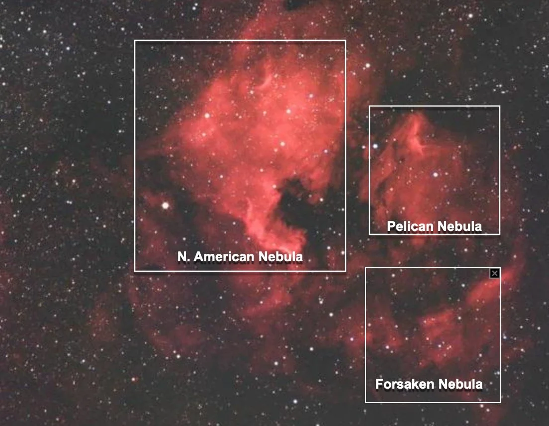
Relationship between the North American Nebula, the Pelican Nebula, and the Forsaken Nebula (Image credit: SkyMap.org)
IC 5068 consists of glowing clouds of ionized hydrogen gas, but with relatively low surface brightness compared to the North America and Pelican Nebulae. This faintness and overshadowing location have kept it less celebrated, but not less interesting!
Also known as LBN 328 and Cederblad 183B, IC 5068 was initially thought to be about 1,600 light-years from Earth in the rich Milky Way star fields of Cygnus. However, recent measurements from the Gaia space observatory have helped pin down the distance to about 2,500 light-years.
It appears in the sky near the star Deneb – the tail of the Swan – though Deneb is not the source of its glow. In fact, IC 5068 is part of the same expansive star-forming complex as the North America and Pelican Nebulae, a giant ionized hydrogen cloud cataloged as Sharpless 2-117.
Like its neighboring nebulae, IC 5068 shines with a characteristic red hue from hydrogen atoms energized by young, massive stars in the region. All of these nebulae are physically connected: essentially, IC 5068 represents the southern extension of the North America/Pelican Nebula H II region, separated visually by intervening dark clouds.
In photographs, IC 5068 appears as a broad, textured patch of nebulosity with dramatic dark dust lanes crisscrossing its field. These obscuring bands of interstellar dust carve the nebula into distinct sections and even help delineate its boundary from the adjacent Pelican Nebula.
The pattern of dark streaks has a striking appearance – astronomy writer Stephen James O’Meara poetically dubbed IC 5068 the “Black Waterfall” for the look of inky rivulets cascading over the nebula’s luminous clouds. The dark lanes in IC 5068 resemble a curtain or waterfall of black silhouetted against the radiant hydrogen gas. When my wife saw this image, she commented that it looked like dark water was running down a pane of glass!
Such dust features represent dense, cool regions of the cloud where new stars may eventually form, even as nearby hot stars light up the surrounding gas.
History:
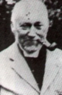
Rev Thomas Henry Espinell Compton Espin (1858-1934)
IC 5068 was discovered in 1899 by the British astronomer Thomas Henry Espinall Compton Espin. Espin found this nebula on September 7, 1899, during a time when long-exposure photography was revolutionizing nebular astronomy. By then, the North America Nebula had been known since William Herschel’s 18th-century surveys, and Max Wolf had photographed the region in 1890, but IC 5068’s faint glow had escaped notice until Espin’s observation.
It was subsequently entered into Dreyer’s Second Index Catalogue (published in the early 1900s) as object number 5068. Being an IC object (rather than an NGC object) highlights how IC 5068 is a later addition to the catalog of nebulae, reflecting its subtle appearance. Despite its cataloging, this nebula remained relatively obscure to most observers for decades, largely “forsaken” in the shadow of its showy neighbors in Cygnus.
Scientific interest:
Although IC 5068 itself hasn’t been the subject of as much individual research as the North America Nebula, it contributes to our understanding of the wider Cygnus star-forming region. Astronomers have found that IC 5068, NGC 7000, and IC 5070 are all portions of one immense H II region – a huge cloud of ionized hydrogen spanning several degrees.
In radio surveys and infrared images, the apparently separate nebulae actually form a continuous cavity of glowing gas and dust, known by the radio designation W80, carved out by stellar winds and radiation. The dark nebulae (such as the prominent lane cataloged as LDN 935 between NGC 7000 and IC 5070) lie in front of parts of this complex and give the illusion that these nebulae are distinct. In reality, IC 5068 marks the southern arc of this vast cloud, sometimes called the “Cygnus Arc.” Deep studies have even identified the likely source of the nebula’s illumination: at least one extremely hot O-type star is hidden behind a dust cloud in this region, and its intense ultraviolet light ionizes the gas of the North America/Pelican/IC 5068 complex. (Deneb, although nearby in the sky, is a foreground star and not hot enough to ionize these nebulae.)
The Annotated Image

Created in Pixinsight using the ImageSolver and AnnotateImage scripts.
The Location in the Sky
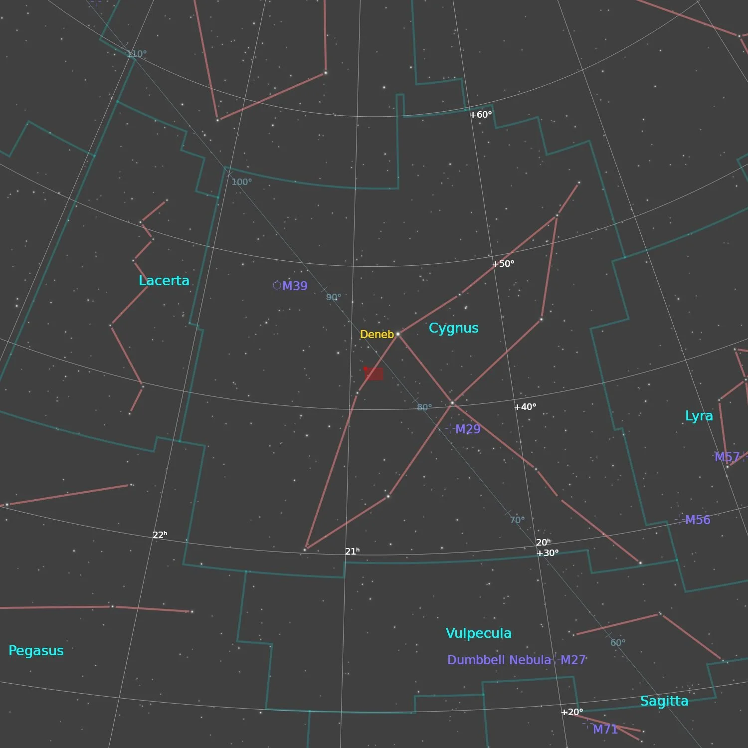
This annotated image created with Imagesolver and FInderChart Scripts in Pixinsight.
About the Project
Picking the Target
We were getting to the time when parts of Cygus were accessible to my observatory location. I do have a string of tall trees on my eastern border, so I have to wait until Cynus targets clear those trees before they are accessible to me.
I have captured a lot of great images in Cynus. It is a rich part of the sky with many bright and famous nebulae. And it has been my happy hunting ground in the past. But now, I often seek out those that are not as well-known and perhaps not shot as often.
One way of doing this is going to the wonderful website, Astrobin.com. Besides being a hub of international Amateur Astrophotography, it has powerful search and exploratory tools. One of those allows you to look at submitted images by constellation.
I did that for Cygnus, and I saw all of my old favorite targets there, but then one I had not heard of popped up - The Forsaken Nebula. It was very faint, but it was also unusual - and as I researched it further, I loved the idea that it was often passed over.
Well, I decided to give this poor neglected target some telescope time to see what I could do with it!
Data Collection
The weather cooperated on July 18, 20, 21, and 23. Well - sort of cooperated. The evenings were often “iffy,” but now that I have an observatory set up and running, it is much easier to start things up as well as shut things back down. Now those “iffy” nights are worth trying. So I went for it. Some nights, I was shut down early as clouds rolled in. But some went the distance.
Many of these nights were surprisingly hot, and a few were much cooler. Because of this, I set the im temp on the camera to -10C. This was a temp that I could still hit even on the hottest days. I opened the observatory around 8 pm to let things cool down. The first 3 nights, I ran narrowband exclusively. Once I felt I had some good data, the last night I added some R, G, and B subs so I could have nicer star colors.
The ASI2600MM-Pro camera was set to use zero gain for the RGB subs and a gain of 100 for the narrowband subs.
After the last night, I shot new Flat Cal frames and planned on using older Dark Cal frames.
Reviewing the Data
I gathered a total of about 15 hours of data. I always blink all of my data before doing any processing. As I did that this time, I saw something unusual. I saw a LOT of frames that were severely impacted by thin clouds. Darn! The clouds snuck in there and I was not even aware of them!
So I culled those frames. Then I ran SubframeDetector and removed a few more frames that had the worst star sizes. The total amount removed added up to a painful 3 hours! Ouch. It’s a shame, but I really don’t want those images going into my integration process!
Processing Overview
I planned on following my standard workflow for narrowband images with RGB stars - a high-level view of this can be seen below.
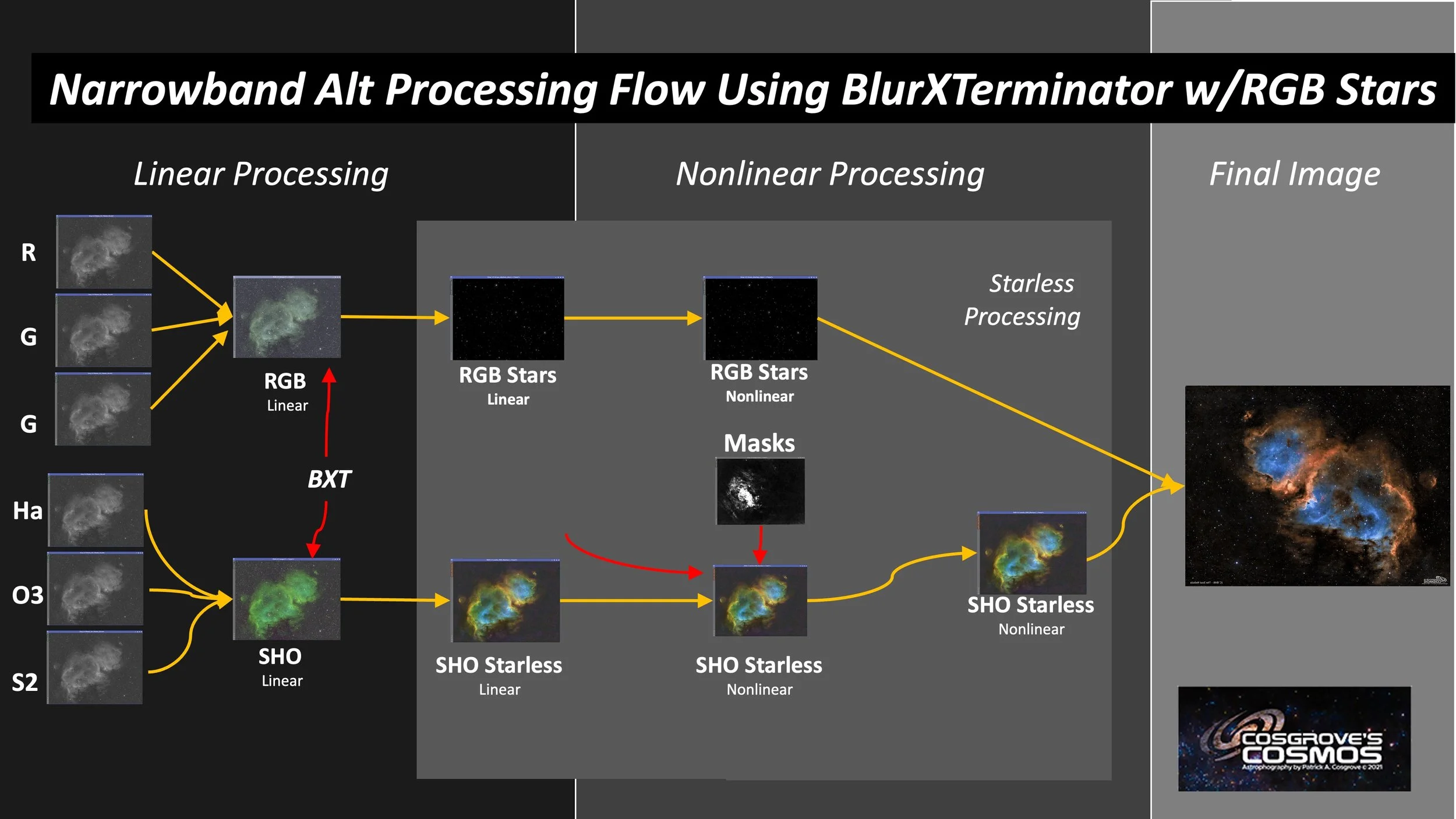
The high level SHO workflow used.
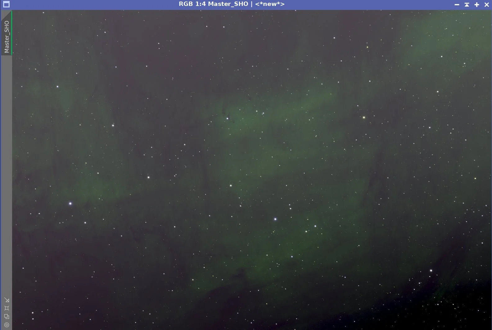
This target is much fainter than the North American or Pelican Nebulae. After almost 12 hours of SHO data, this was my initial starting image. There is not a lot of signal there!
The initial SHO nonlinear image. (click to enlarge)
But even here, you get a sense of the thinness and transparency of the nebla. I really wanted to try to preserve this quality of the image.
I ended up having problems with my color handling of the SHO image.
Lately, I have been using the NarrobandNormalization process for this. But this time, I couldn't achieve the color and tone scale I was looking for. The brighter areas were coming out too bright and blocked up, and the darker areas were too dark.
So, I went back to my old manual method of dealing with the strong greens of an initial SHO image. But this was no better.
I started to think about how I might go about this differently. Then I had a thought - when I process RGB images, I always use SPCC to get the color and tone scale about right. I don’t do that for narrowband. After all, what is the true color of an SHO image? Just about whatever you want it to be! So I don’t use SPCC there.
However, I could.
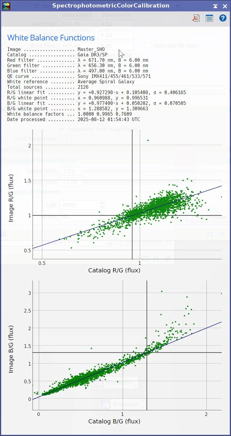
SPCC does have a narrowband mode. You put it in that mode, enter the specs on your narroband filters, click calibrate, and run it. So I tried this for the very first time. The regression curve came out looking pretty good, but the “corrected” image did not look promising at all
This is what I saw after running SPCC:
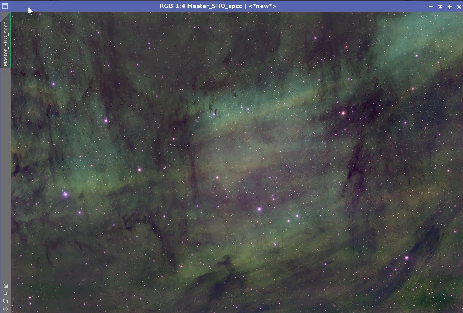
After Narrowband SPCC - Yike! (click to enlarge)
I almost gave up, but then I hit the radiation button on the STF panel to redo the screen mapping and the image changed to this:
After an STF update!
Wow - this is what I was looking for!
After getting to this point, the image almost processed itself. Simple. Easy. Relatively few steps.
Compared to my last image - the Cat’s Eye Nebula - this was a piece of cake! That one came into the world kicking and screaming the whole way.
This one came into the world quickly and easily!
Look below for the complete step-by-step processing walkthrough! Note: This walkthrough is based on Pixinsight.
Final Results
I am delighted with my final result. This is such an interesting image. Light and airy with wonderful colors and details.
This is one of those images that must really be seen on the large screen to best appreciate the fine details of the Black Waterfall in the image foreground.
This is now one of my favorites. I hope you like it as well!
More Information
📌 Target Details & Planners
https://theskylive.com/sky/deepsky/ic5068-object — Object page with coordinates, visibility tools, and finder charts for planning sessions from your location.
https://spider.seds.org/ngc/ngc.cgi?i5068= — SEDS NGC/IC entry with RA/Dec, size, Dreyer notes, and quick links to DSS/SIMBAD/ADS.
https://www.docdb.net/show_object.php?id=ic_5068 — Compact catalog sheet with cross-IDs (Ced 183b, LBN 328), dimensions, and references.
https://www.wikisky.org/starview?locale=EN&object_id=255&object_name=IC+5068&object_type=3 — Interactive sky view centered on IC 5068 for framing and star-field context.
🕰️ History & Cataloguing
https://cseligman.com/text/atlas/ic50a.htm — C. Seligman’s IC 5050–5099 notes; IC 5068 entry with discoverer attribution and historical comments.
https://haroldcorwin.net/ngcic/ — Harold Corwin’s historically-aware NGC/IC notes, identification corrections, and catalogue history background.
https://de.wikipedia.org/wiki/IC_5068 — Brief IC 5068 page (German) listing object type, discoverer (T. H. E. C. Espin), discovery date, and catalog cross-IDs.
https://en.wikipedia.org/wiki/T._H._E._C._Espin — Bio of Rev. T. H. E. C. Espin, credited with the 1899 discovery referenced in IC notes.
🔬 Science of the Region (W80 / North America–Pelican Complex)
https://www.aanda.org/articles/aa/pdf/2005/05/aa1788.pdf — Comerón & Pasquali (2005): identifies a hidden O-type star as the ionizing source for the NAP/W80 complex.
https://ri.conicet.gov.ar/bitstream/handle/11336/22324/Cersosimo_2007_ApJ_656_248.pdf?isAllowed=y&sequence=1 — Cersósimo et al. (2007): radio recombination line work constraining distance and structure for W80.
https://arxiv.org/abs/1702.05999 — Damiani et al. (2017): X-ray survey of the North America–Pelican star-forming region; young stellar population and clustering.
💡 Interesting Notes & Free Media
https://www.astronomy.com/picture-of-the-day/photo/the-forsaken/ — Astronomy.com’s Picture of the Day: origin of the “Forsaken/Black Waterfall” nicknames and location context.
https://skyandtelescope.org/online-gallery/the-forsaken-nebula/ — Sky & Telescope gallery write-up with a concise explainer of the dark “waterfall” dust lanes.
https://commons.wikimedia.org/wiki/Category:IC_5068 — Wikimedia Commons category with public-domain/CC-licensed media (check individual file licenses).
https://skyandtelescope.org/online-gallery/ic-5068-the-forsaken-nebula-2-panels-mosaic/ — Another S&T gallery entry highlighting the dust-lane structure and proximity to NGC 7000/IC 5070.
Capture Details
Lights Frames
Taken the nights of July 18, 20, 21, and 23, 2025
39 x 300 seconds, bin 1x1 @ -10C, Gain 100, Astronomiks 6nm Ha - 36mm unmounted
45 x 300 seconds, bin 1x1 @ -10C, Gain 100, Astronomiks 6nm O3 - 36mm unmounted
39 x 300 seconds, bin 1x1 @ -10C, Gain 100, Astronomiks 6nm S2 - 36mm unmounted
23 x 90 seconds, bin 1x1 @ -10C, Gain 0, ZWO Red - 36mm unmounted
21 x 90 seconds, bin 1x1 @ -10C, Gain 0, ZWO Green - 36mm unmounted
20 x 90 seconds, bin 1x1 @ -10C, Gain 0, ZWO Blue - 36mm unmounted
Total - after culling bad subs - of 1 1 hours and 51 minutes.
Cal Frames
30 Darks at 90 seconds, bin 1x1, -10C, gain 0
30 Darks at 300 seconds, bin 1x1, -10C, gain 100
30 Dark Flats at Flat exposure times, bin 1x1, -10C, gain 100 fro narrowband, gain 0 for broadband
One set of Flats done:
15 Ha Flats
15 O3 Flats
15 S2 Flats
15 R Flats
15 G Flats
15 B Flats
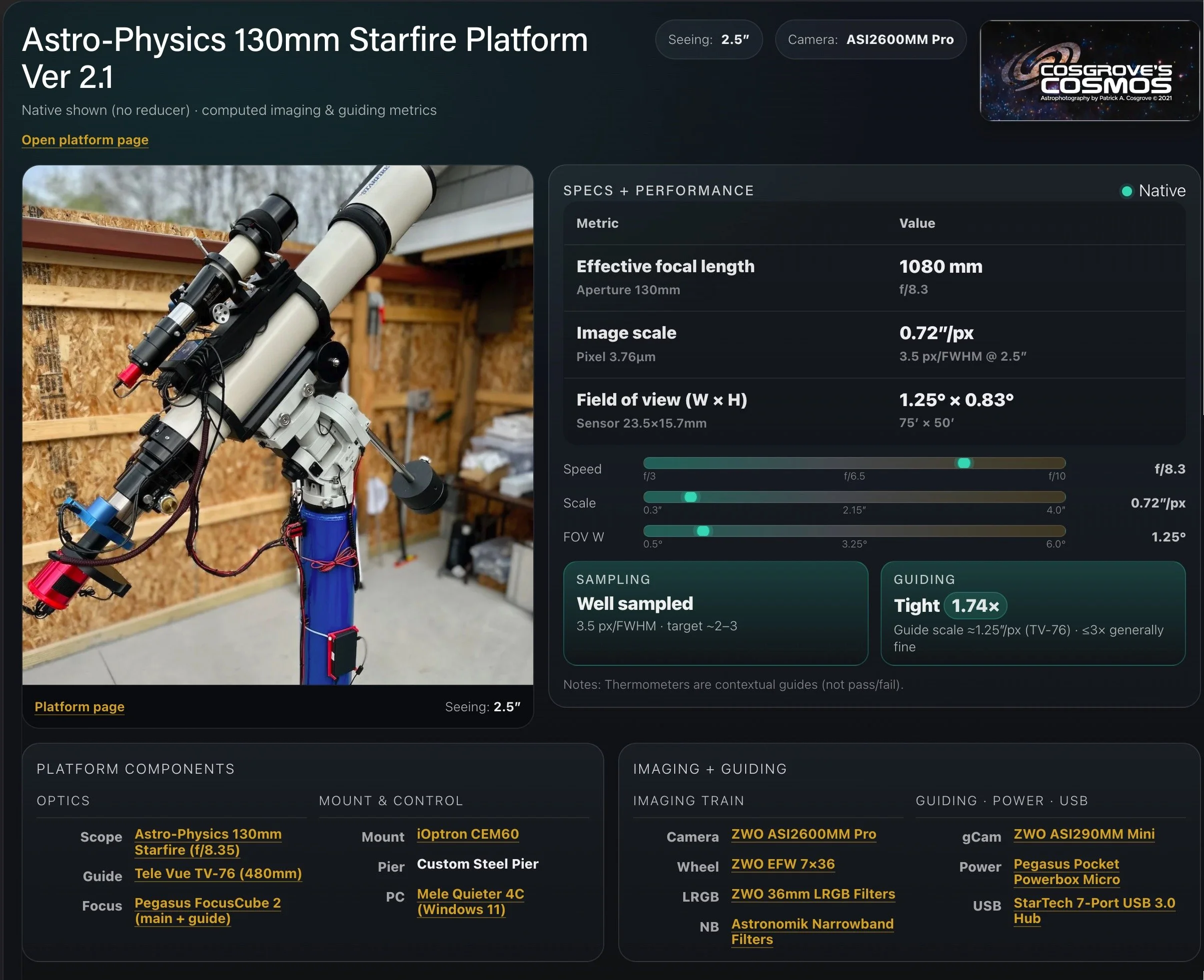
Platform used for this project
Software
Capture Software: PHD2 Guider, NINA
Image Processing: Pixinsight, Photoshop - assisted by Coffee, extensive processing indecision and second-guessing, editor regret, and much swearing…..
Image Processing Walkthrough
(All Processing is done in Pixinsight, with some final touches done in Photoshop)
1. Blink
Ha
14 frames removed for clouds
O3
10 frames removed for clouds
S2
13 frames removed for clouds
Red
No frames removed!
Green
3 Frames removed for clouds.
Blue
3 Frames removed for clouds.
Darks
All looks ok
Dark Flats
All looks ok
Flats
all good
2. SubFrameSelector
Ha:
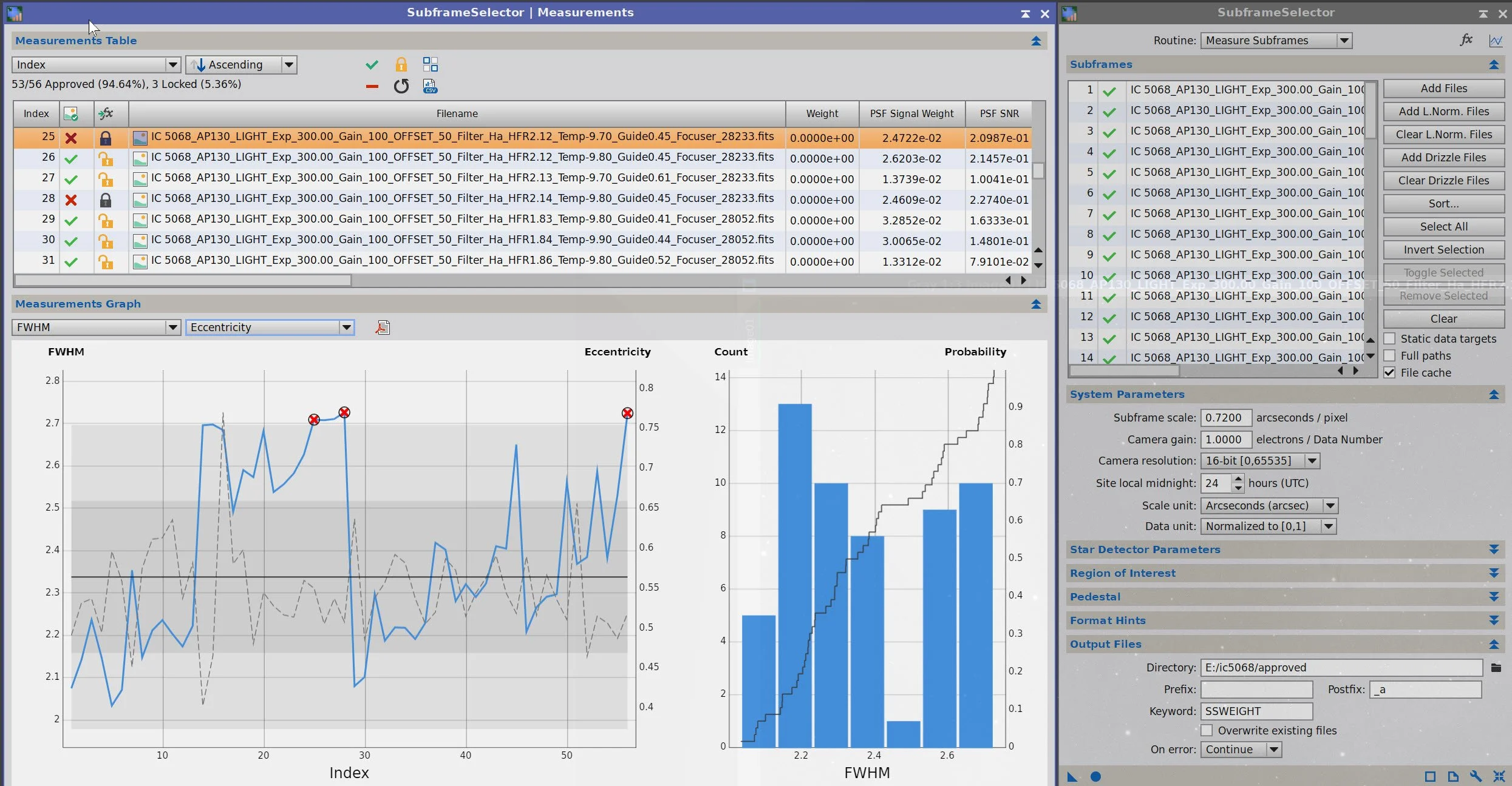
3 more frames removed.
O3:
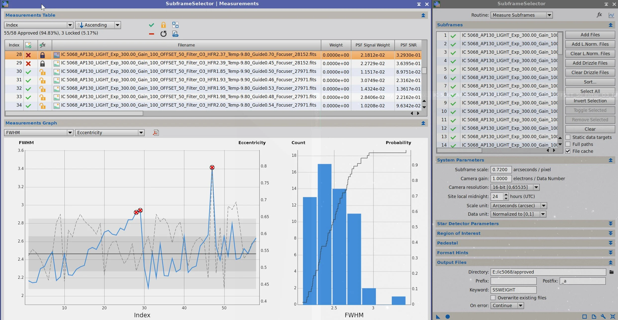
3 more frames removed
S2:
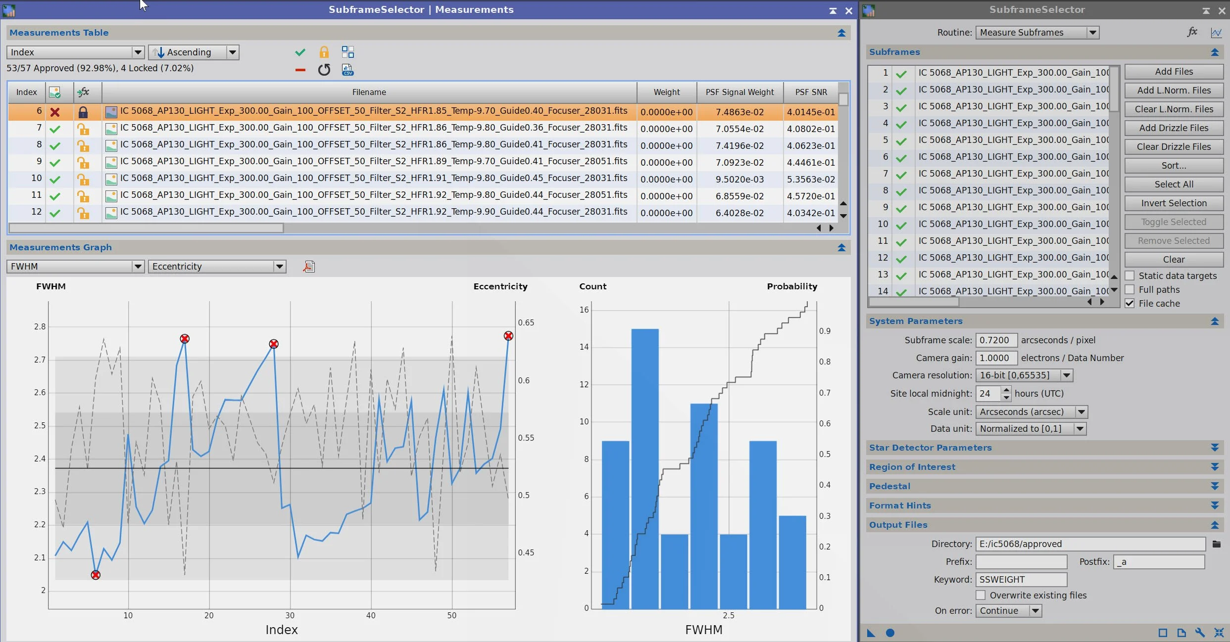
4 more frames removed
Red:
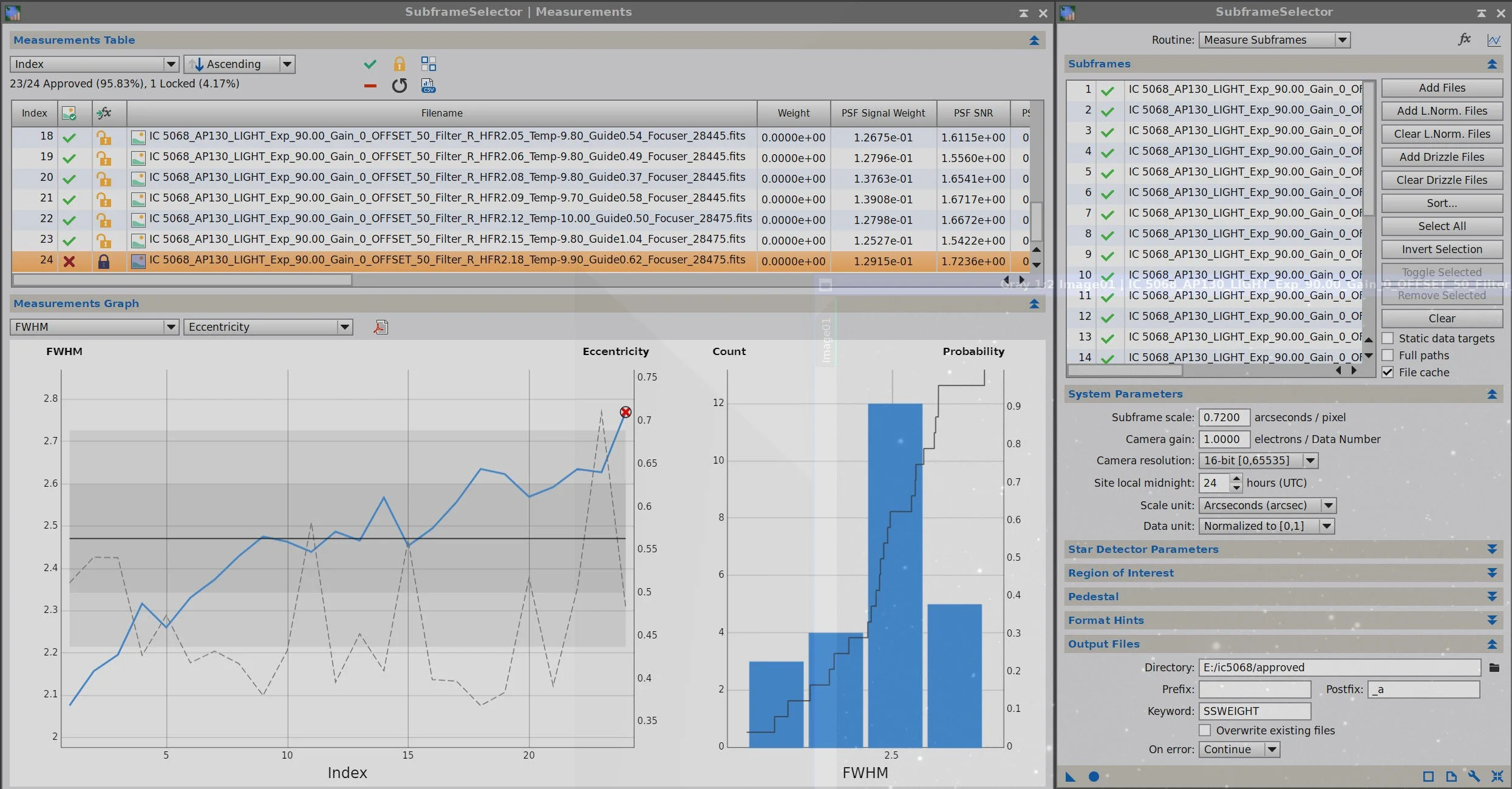
One more frame removed.
Green:
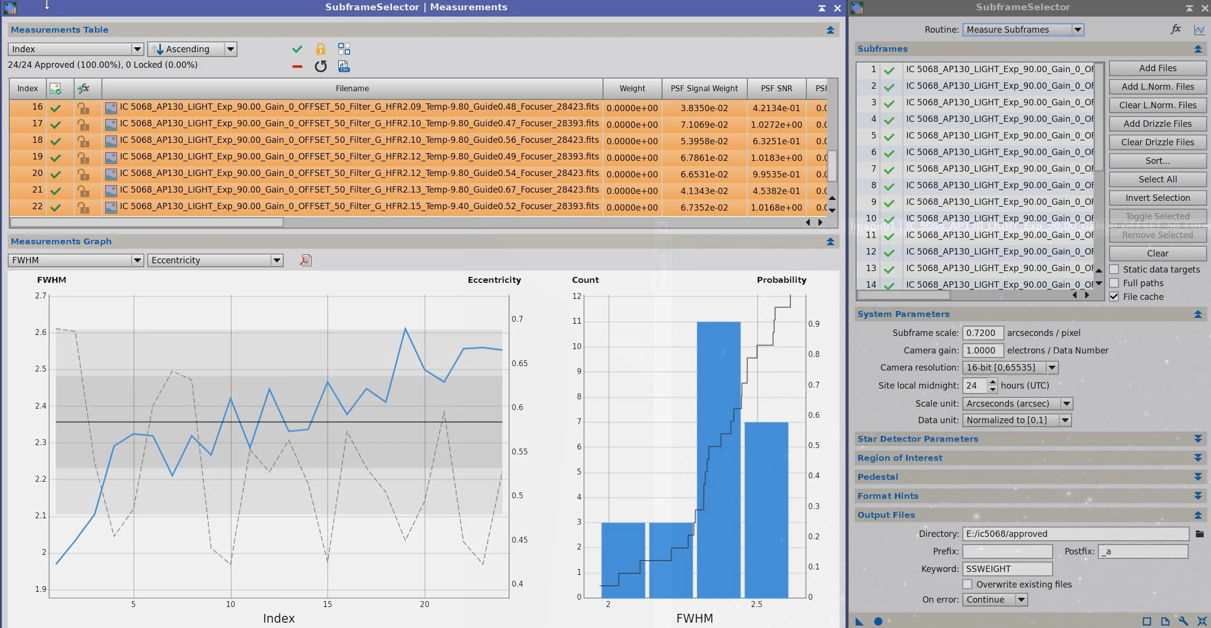
No more frames removed.
Blue:
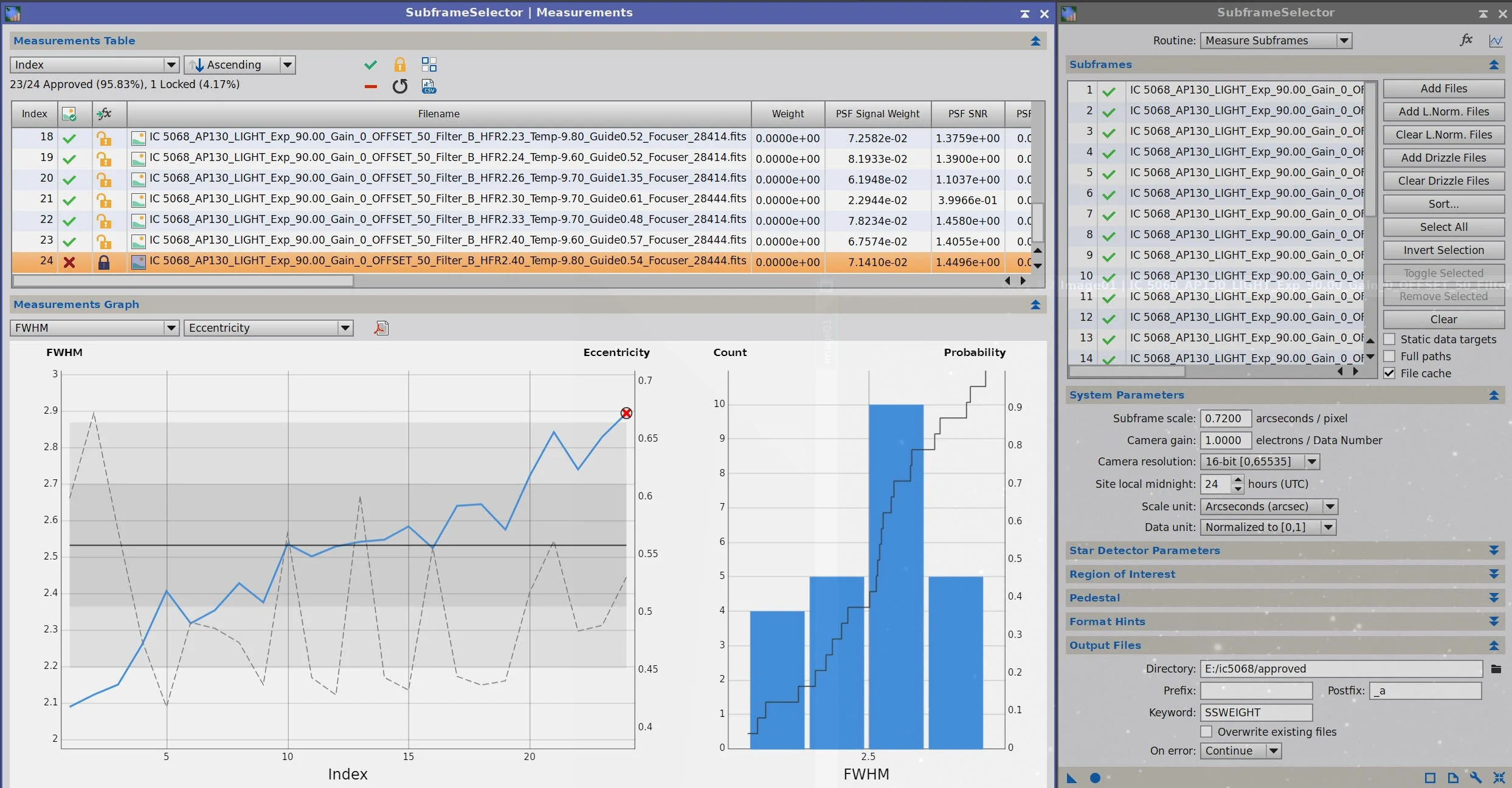
One more frame removed.
3. WBPP 2.8.9
Reset everything
Load all lights
Load all flats
Load all darks
Select - maximum quality
Reference Image - auto - the default
Select the output directory to wbpp folder
Enable CC for all light frames
Pedestal value - auto
Darks -set exposure tolerance to 0
Lights - set exposure tolerance to 0
Lights - all set except for a linear defect
set for Autocrop
WBPP run 3 minutes - no errors

WBPP Calibration View
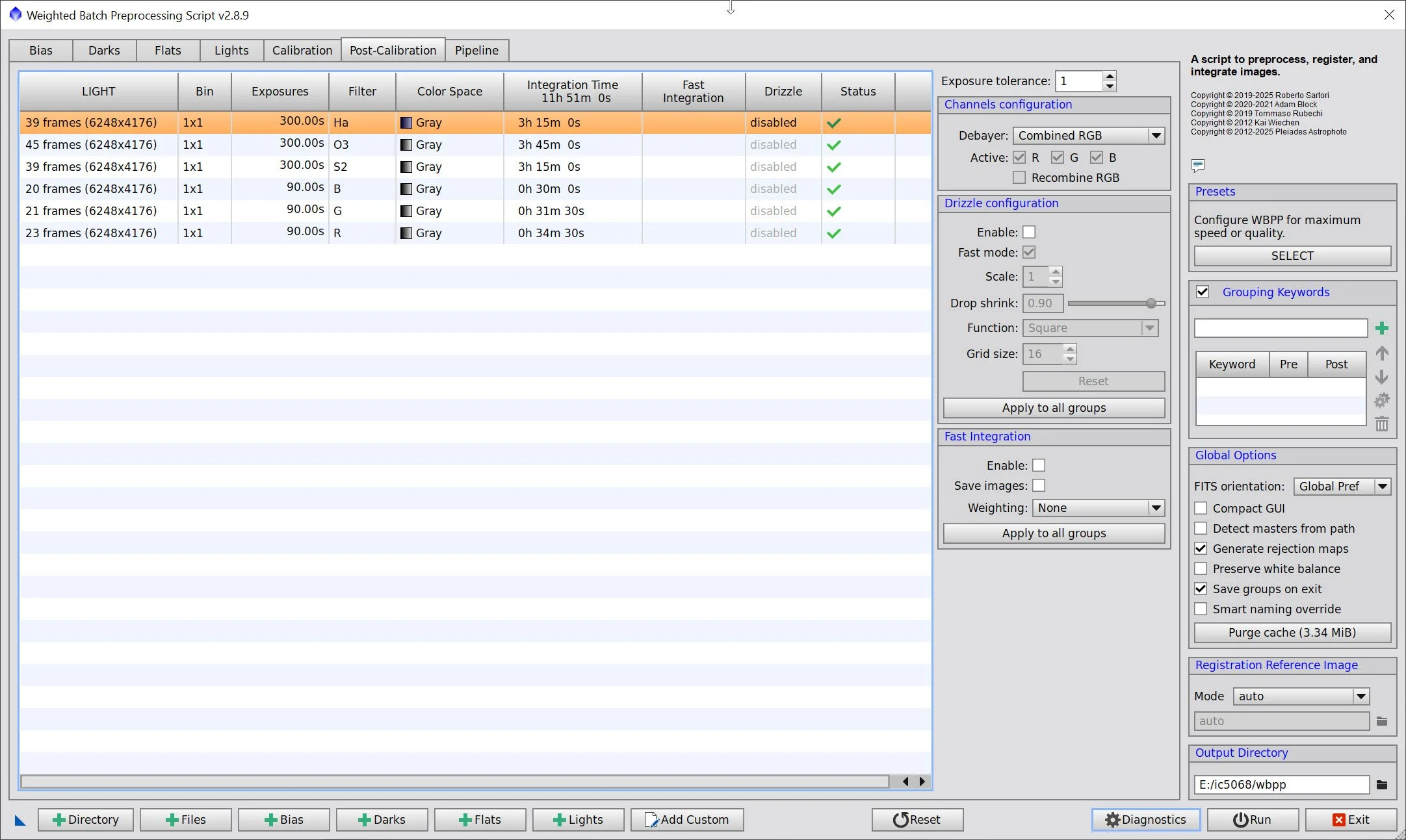
WBPP Post Calibration View

WBPP Pipeline View
4. Load Master Images and Create Color Images
Load all master images and rename them.
Using CombineChannels, create the Master SHO image
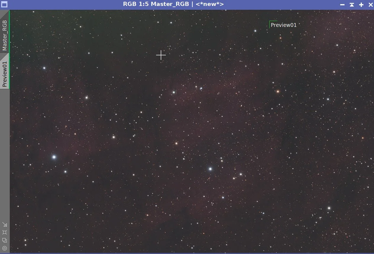
Using CombineChannels, Create the Master RGB image
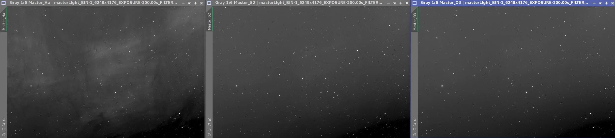
Master Ha, O3, and S2 images
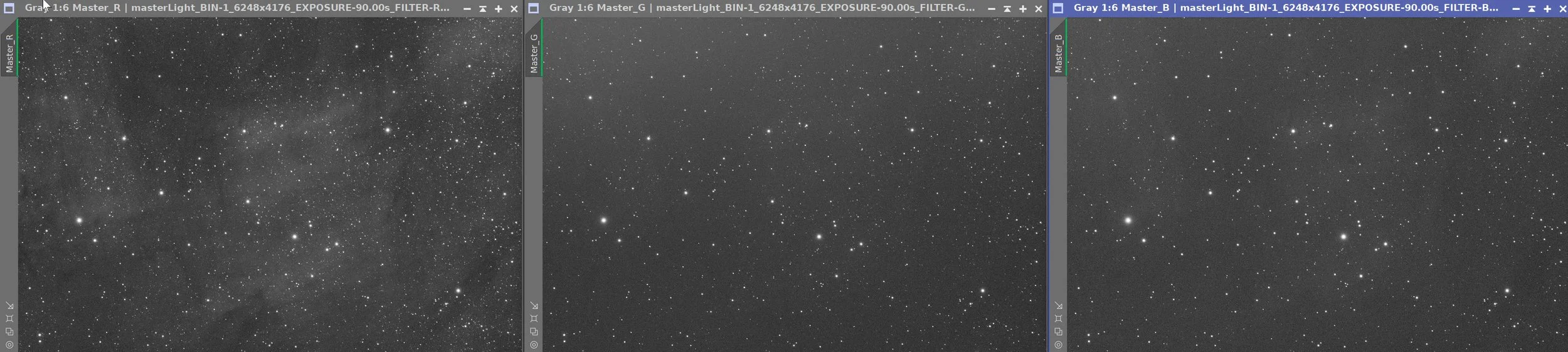
Master R, G, & B images
Master SHO Image (click to enlarge)
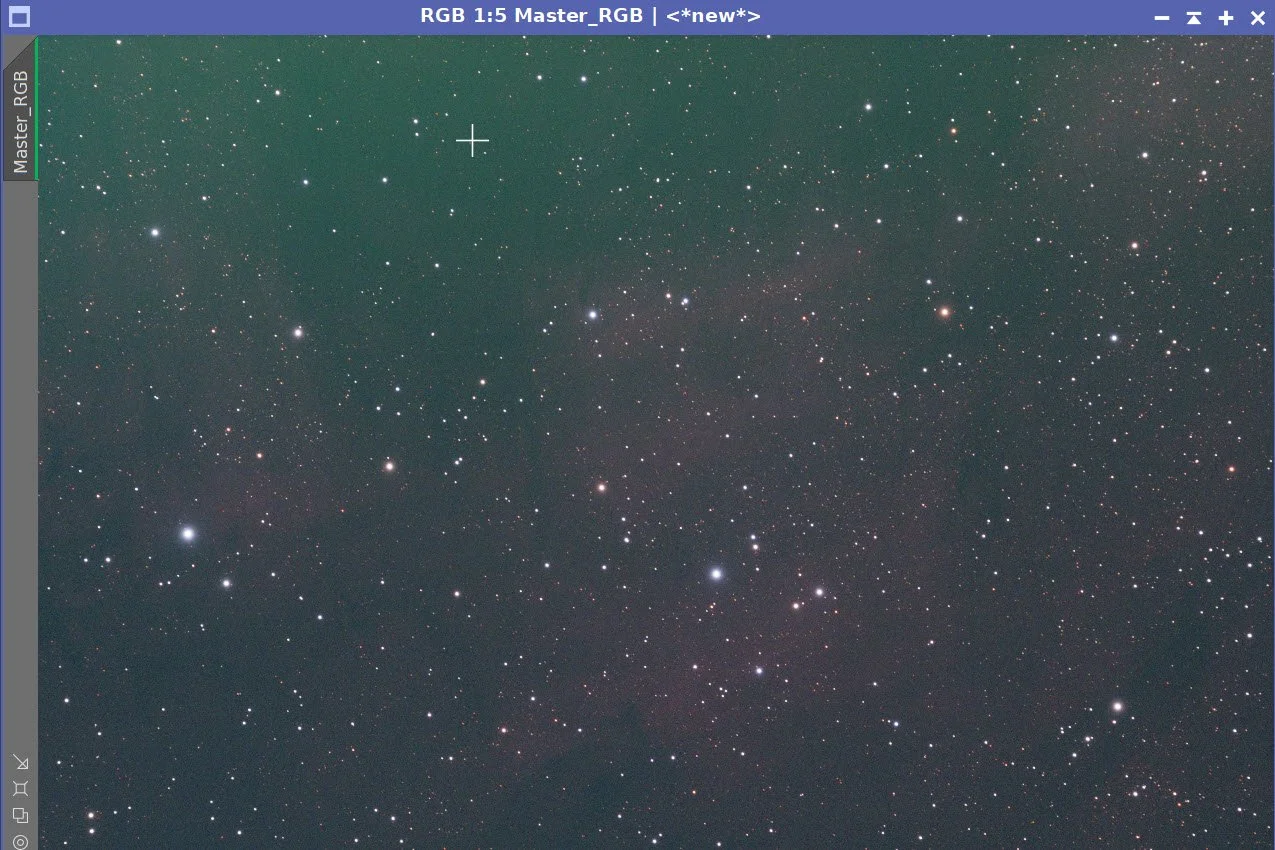
Master RGB Image (click to enlarge)
5. Initial Process of Linear RGB data
Run DBE for the RGB linear image. Use subtraction for the correction method. Choose a sampling plan that avoids the nebulae.
Run BXT - correct only. This cleans up and stars at the corners.
Select a preview rectangle sampling the background sky and then set up and run SPCC.
Use the 571 device curve
Use ZWO R, G, & B filter curves,
Run Full BXT - I am using default values here as I do not want to shrink the stars too much - I want them bigger to be better seen through all of the narrowband nebulae.
Run NXT V3 - see params from snapshot below
Run SXT and save the RGB stars.
Master RGB Before Image (click to enlarge)
Master RGB Sampling Plan (click to enlarge)
Master RGB after DBE (click to enlarge)
Master RGB Background (click to enlarge)
The initial RGB Image (click to enlarge)
Master_RGB After SPCC (click to enlarge)
SPCC Regression Result (click to enlarge)
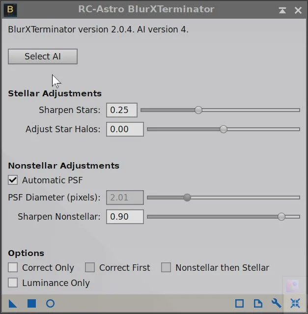
BXT Parameters used.
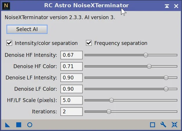
NXT Parameters used.


Master RGB Before BXT Correct Only, After BXT Correct Only, After SPCC, After BXT Full, After NXT V3
Final Linaer RGB image.
Master RGB Stars Only
6. Process the Linear SHO Data
Run DBE for the SHO linear image. Use subtraction for the correction method. Choose a sampling plan that avoids the nebulae.
Run BXT - correct only. This cleans up and stars at the corners.
RUN PFSImage to get the star sizes. X = 1.81, Y= 1.92
Run Full BXT -I used values very close to the measured star sizes. See the panel snapshot below for the params used.
Run NXT V3 - see params from snapshot below.
I had a lot of trouble getting the color I wanted from this image. I tried manual methods and the NarrowbandNormalization script, but I couldn’t achieve the desired result. Then I had a thought. SPCC can be used with Narrowband images, but I had never tried it. When I gave it a go at first, I thought it looked terrible! All dark Green! But then I did an STF Update, and suddenly there was the image I had been looking for!
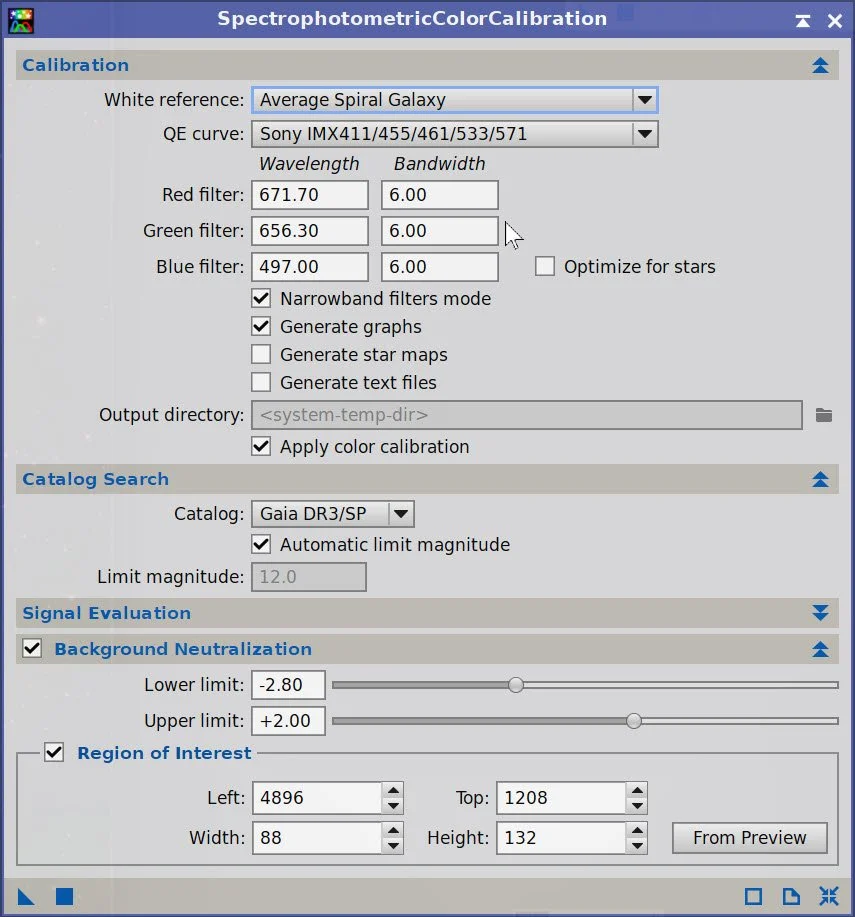
Select a preview rectangle sampling the background sky and then set up and run SPCC.
Use the 571 device curve
Define the filter specs from my Astronomiks narrowband filters.
Check Narrowband mode
Check the color calibration box.
Run
Update STF on the new image.
Run SXT and save the RGB stars.
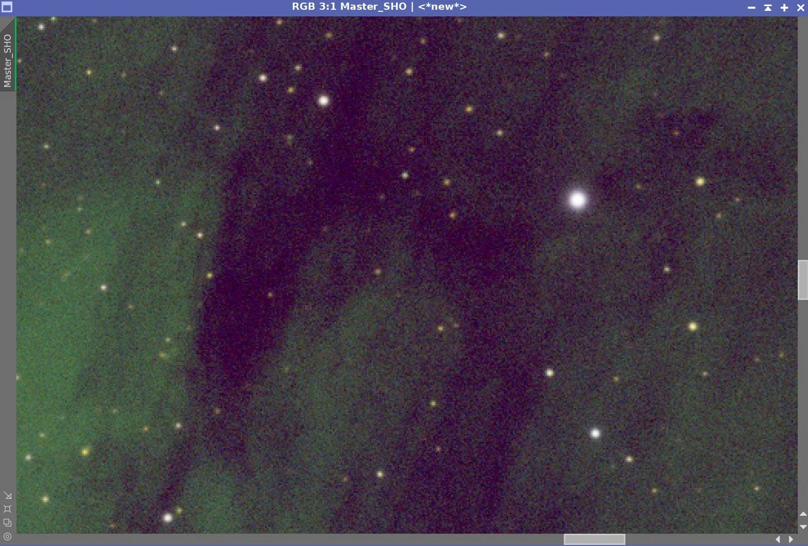
Starting SHO Image.
Before DBE (click to enlarge)
Mastr SHO DBE Sample Patern (click to enlarge)
SHO after DBE and fresh STF. (click to enlarge)
SHO background removed (click to enlarge)
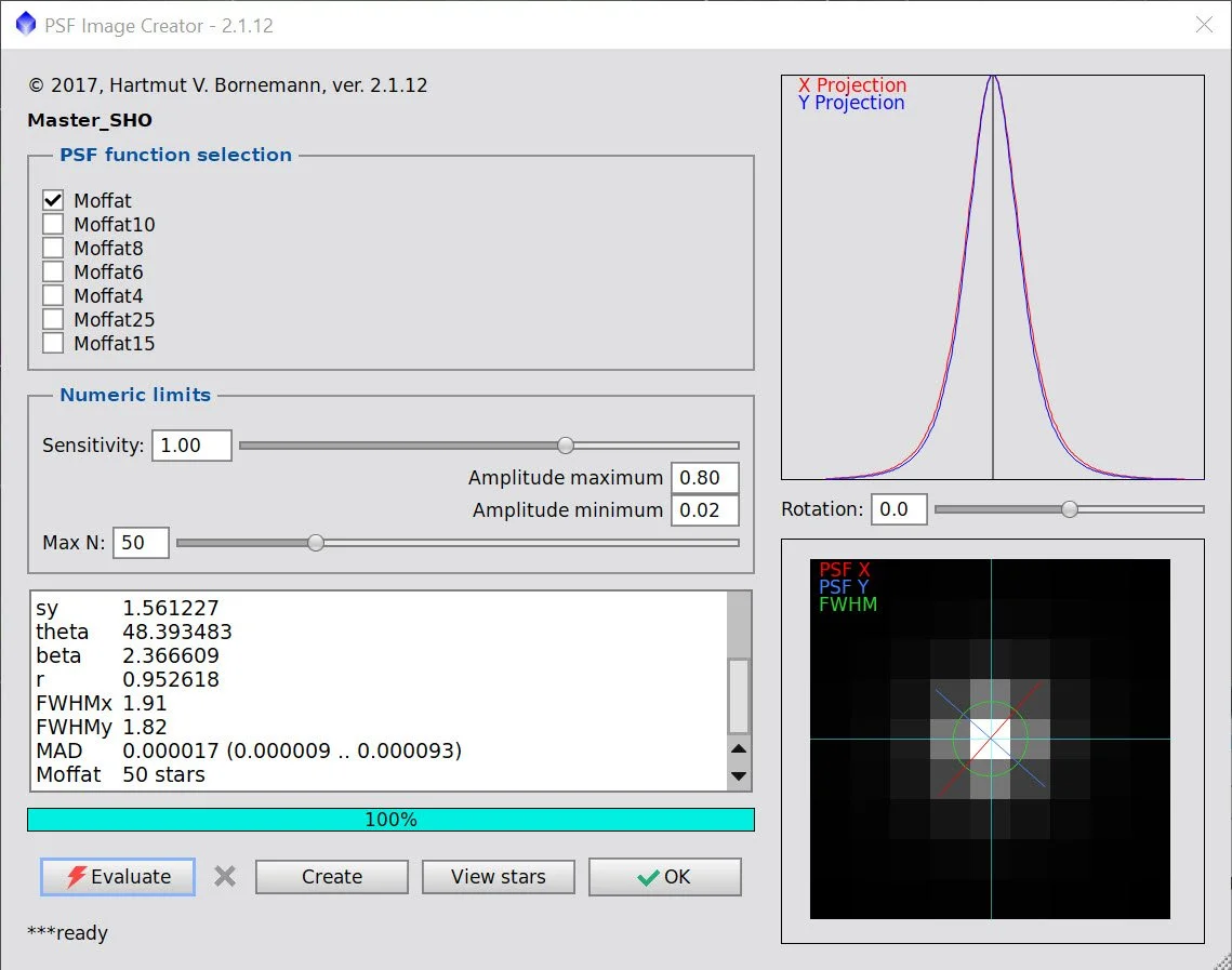
Results from PFSImage
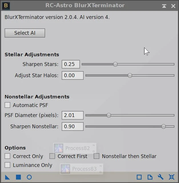
BXT Params Used
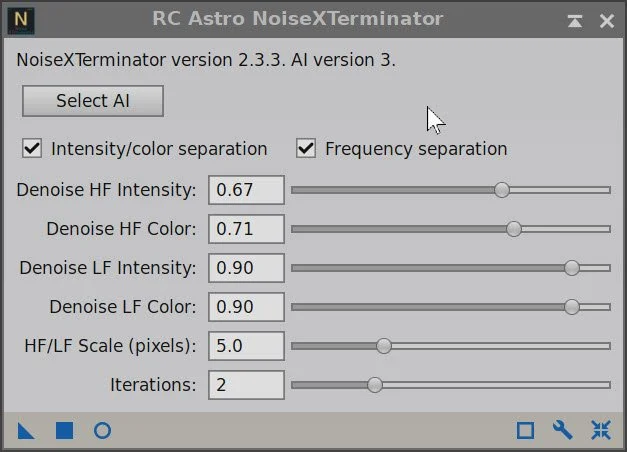
NXT V3 params used.


Master SHO before BXT Correct Only, After BXT Correct Only, After BXT Full, After NXT V3
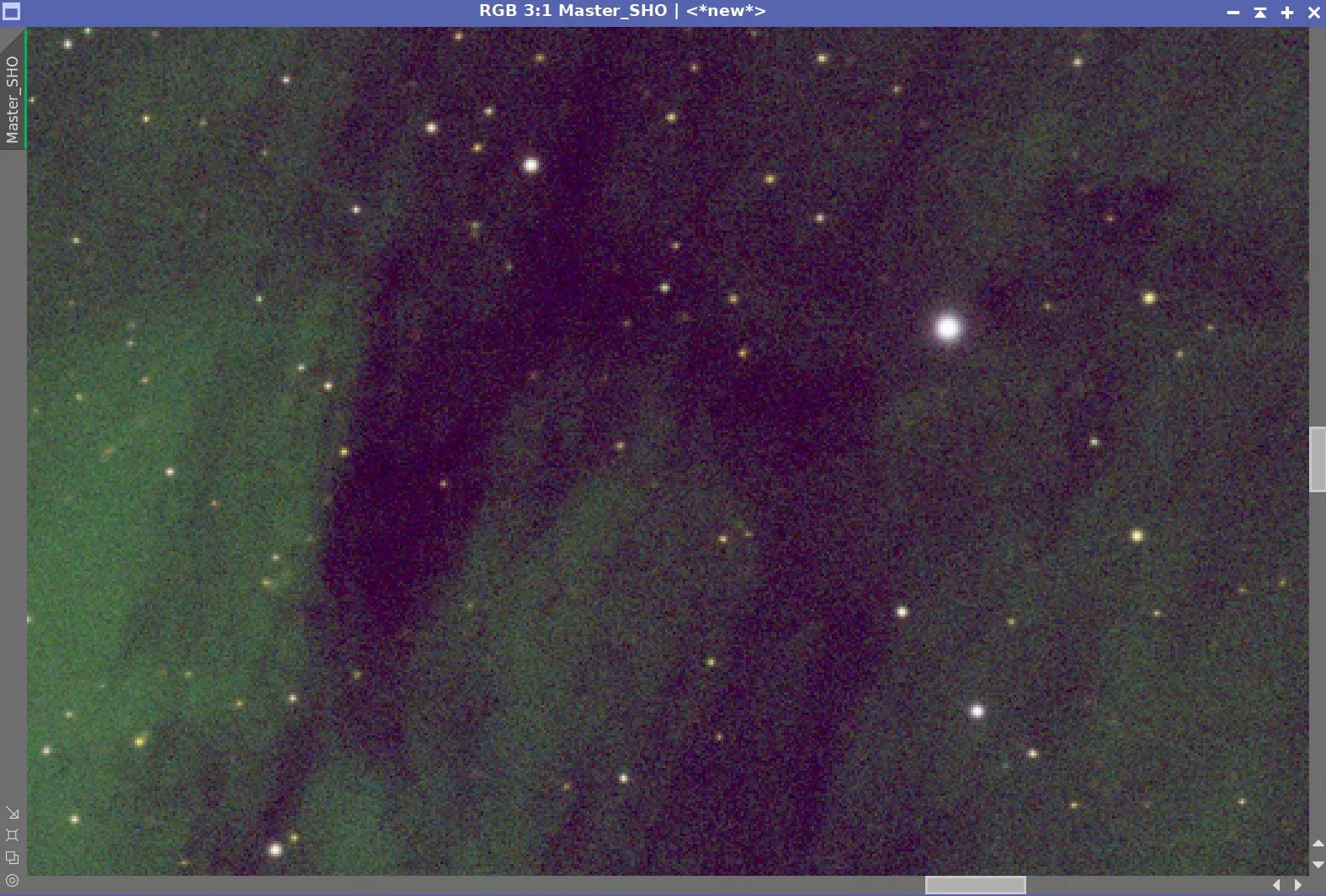
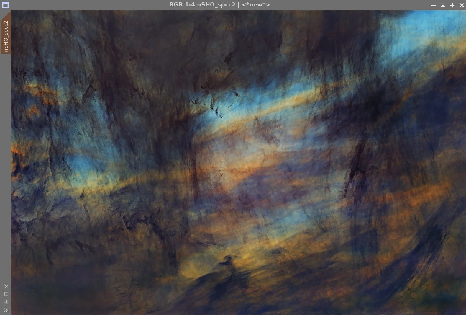
Master SHO After SPCC but before STF update (click to enlarge)

Master SHO image After STF Update (click to enlarge)

Master SHO starless after STX
7. Process the SHO Starless Image
Take the image Nonlinear using the STF->HT method
Run SCNR Green at 0.8 to remove the green cast
Now we have magenta backgrounds to deal with:
Invert the image
Run SCNR Green at 0.8 again.
Invert the image back.
Now I applied a CT to darken the shadow regions and brighten the highlights - also to boost overall saturation.
Now I need to bring out the finer details. I chose LHE to do this.
Radius of 40, contrast limit of 2.0, Amount of 0.22, and an 8-bit histogram
Another CT to darken and boost contrast
Now do an MLT sharpen - see panel snapshot below for settings below.
Another CT to tweak things
Now - let's handle noise. NXT V3 is using settings from the panel snapshot below.
I still have too much magenta in the shadows and other areas.
Create a Magenta Mask using ColorMask_Mod Script
Blue is using Bill Blanshan’s Mask Blur Script.
Apply mask
Use CT to adjust saturation on masked areas.
The initial nonlinear SHO Starless image (click to enlarge)
After Inverting the SHO image. (Click to enlarge)
Invert again. Magenta mostly gone! (click to enlarge)
After LHE to bring out faint detail (click to enlarge)
MLT Sharpening Panel (click to enlarge)
Another CT adjust. (click to enlarge)

After SCNR Green at 0.8 (click to enlarge)
Run SCNR Green at 0.8 again (click to enlarge)
CT to Darken shadows and boost overal saturation (click to enlarge)
Another CT to again darken and boost sats (click to enlarge)
After MLT Sharpening (click to enlarge)
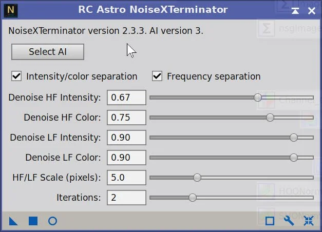
NXT Params used.
After NXT
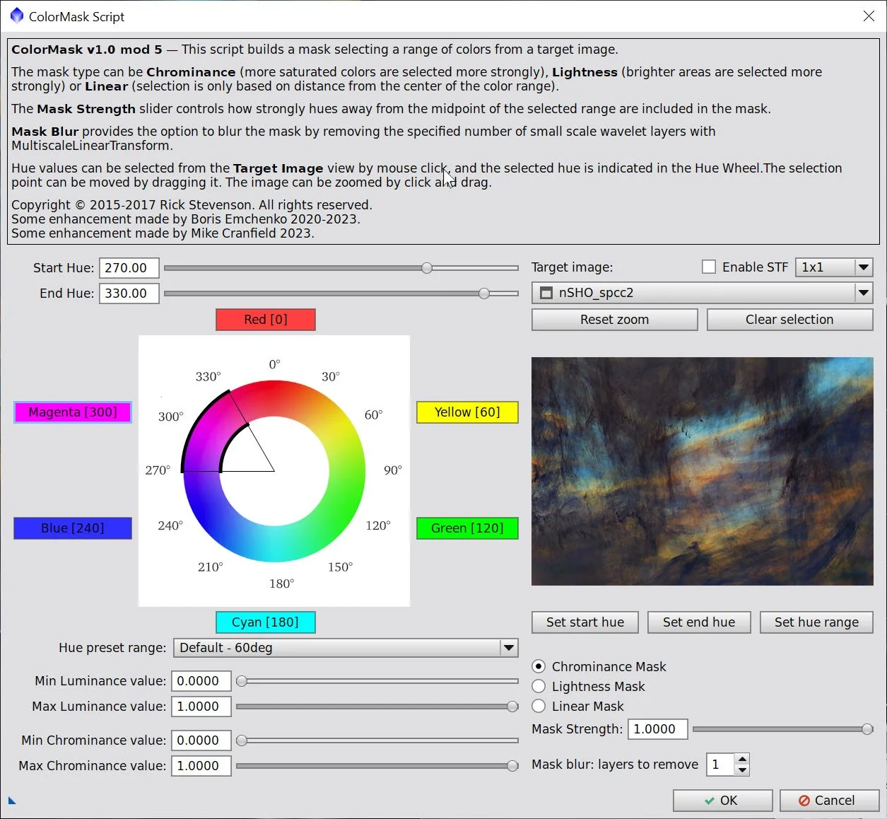
Creating the Magenta Color Mask.
Magenta Mask after blur operation (click to enlarge)
Initial Magenta Mask (click to enlarge)
CT to remove saturation with Magenta Mask in place (click to enlarge)
8. Add The Stars Back In
Use the ScreenStars Script to add the stars back in.
The Final RGB Stars Image (click to enlarge)
The Final Starless SHO image (click to enlarge)
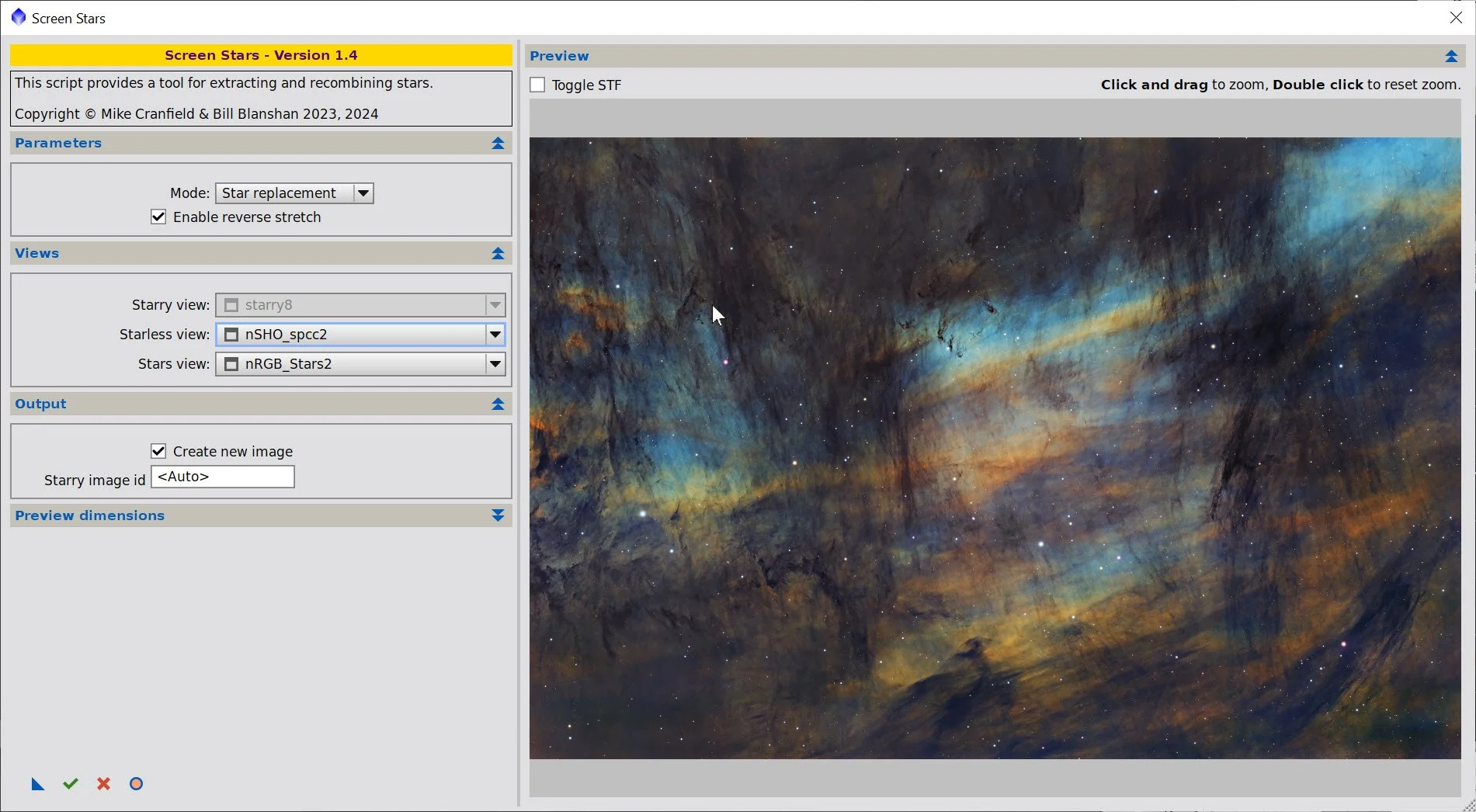
ScreenStars Panel.

The image with Stars inserted!
9. Export the Image to Photoshop for Polishing
I am pretty happy with the image and ready to polish it in Photoshop.
Save the image as a TIFF 16-bit unsigned and move to Photoshop
Make final global adjustments with Clarify, Curves, and the Color Mixer - slight tweaks really
Run Clarifier on the bottom-left corner and top center to get better definition. Areas selected with a lasso with a 100 pixel feather.
Added Watermarks
Export Clear, Watermarked, and Web-sized jpegs.
The Final Image!