
SH2-101 - A Reprocess of The Tulip Nebula - 12.8 Hours in SHOrgb
Date: July 20 2023
Cosgrove’s Cosmos Catalog ➤#0125

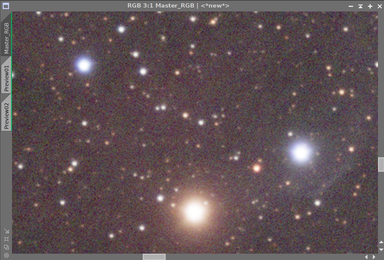
My Reprocess of SH2-101 - The Tulip Nebula (click image for full resolution via Astrobin.com)
Table of Contents Show (Click on lines to navigate)
Another Reprocessing Project
2023 has continued to be a terrible year for Astrophotography. Weather conditions and smoke plumes from the extensive wildfires in Canada continue to block the skies and prevent me from capturing new data!
So while waiting for the heavens to re-open, I am taking some time to revisit data from projects in the past and reprocessing them.
My goal is to see how much better I can do with the same data set now that I have more experience, new and advanced processing tools, and better processing strategies.
In general, I have been super happy with the improvements I have made. But judge for yourself. The image at the top of the page is my new one. Below see the old one.

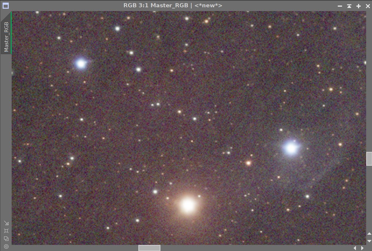
My Original Image. Compare with the image at the top of the page. Which do you think is better?
The original imaging project can be seen HERE.
About the Target (unchanged from the original posting)
Sharpless 101 (specifically Sh2-101) is also known as the Tulip Nebula and is located approximately 6000 light-years away in the constellation of Cygnus (The Swan). Stewart Sharpless first cataloged this rich H II emission region in 1959 in his second catalog of nebulae. Early photographic images of this area resembled a flower, giving rise to its common name.
Most of the targets I have imaged so far have come from the much more familiar Messier Catalog or the NGC catalog - I believe this is the first target from the Sharpless catalog. Wikipedia provides some background on this:
"In 1953 Stewart Sharpless joined the staff of the United States Naval Observatory Flagstaff Station, where he surveyed and cataloged H II regions of the Milky Way using the images from the Palomar Sky Survey. From this work, Sharpless published his catalog of H II regions in two editions: the first in 1953, with 142 nebulae, and the second and final edition in 1959, with 312 nebulae."

Artist rendition of Cygnus X-1 (PBS/Nova Teaching Material Collection)
Also in this region is the first black hole ever discovered, Cygnus X-1!
First detected in 1964 from an X-ray instrument sent aloft on a sounding rocket, Cygnus X-1 was the brightest X-ray source seen from Earth.
In 1971, radio signals were detected, which were used to locate the x-ray source from a star known as HDE 226868. This star is a supergiant but cannot produce the energetic X-rays seen alone. It was concluded that HDE 226868 must have a dark companion with the ability to heat gases in the system to the millions of degrees of temperature necessary to produce X-rays. Measures of Doppler shift in the spectrum of HDE 226868 allowed the star's orbits and its dark companion to be determined. Based on the mass required for these observed orbits - and the fact there was no light signature from its companion - it was proposed that Cygnus X-1 was indeed a back hole - potentially the first-ever detected!
In 1974, Kip Throne famously bet Stephen Hawking that Cygnus X-1 was a black hole. In 1990, Hawkings conceded that X-1 was a black hole, and Throne won the bet.
Wikipedia: Thorne-Hawkings Bet (note: the X-1 bet is described at the end of this link)
It is now believed that Cygnus X-1 is pulling gas from its companion toward its event horizon. This superheated spinning disk of gas is the engine that produces the X-rays seen from Earth.
I have indicated the location of the binary pair on the annotated version of this image below.
The Annotated Image

Annotated version of Sh2-101 created with Pixinsight ImageSolve and AnnotateImage scripts. Note the reference note on the right - in orange - indicating the location of Cygnus x-1.
The Location in the Sky

This annotated image created with Imagesolver and Annotate Image Scripts in Pixinsight. Note the Cygnus X-1 features in red.
About the Project
It is now July of 2023 - and thus far, I have only had two nights where I have been able to collect data. That data was limited and still tainted by wildfire smoke.
So to keep busy, I have been selecting data from old projects and reprocessing them.
Can I take this data and make a better image today than I did then?
And the answer to this question is a resounding ‘YES!”.
I have reprocessed several images so far and have been surprised by how much better they have turned out!
These efforts have resulted in a publication where the initial image was rejected. And on M27, I achieved my first NASA APOD image, and the first image published in all publications it was submitted - a Grand Slam!
Another benefit is that I had not yet started documenting the processing path on the older images. Once I complete the reprocessing effort, I can document the processing for this target.
Target Selection
So why choose the Tulip Nebula for a Reprocess effort?
I was taken soon after I started working on narrow band
It was one of my earliest long integrations -almost 13 hours!
The image I produced from this data was - well - disappointing. I thought I would get a better result from such long integration. Every time I have looked at it - it just struck me as a bit wrong. I did not know why, but it has always gnawed at me a bit!
This is a pretty cool object - and the fact that the Cygnus X-1 Bow wave is in the field of view makes it even more remarkable in my book!
This project never had a processing walkthrough - it was done before I ever started that. So by doing this now, I would be able to add this to my collection.
There is always this idea that somewhere in that data is an image that would be good enough for publication. Perhaps my reprocessing of this data would release this hidden image.
Data Collection
I will let the previous imaging project post discuss these issues. I assume the data is there and will start from scratch using it. For more planning and data collection background, please review the previous post HERE.
Image Processing
What will I do differently with this processing run than the last?
I had collected 30-second subs of RGB star data but never used it with the original image. This time around, I will add the RGB stars!
I will be taking advantage of BlurXTerminator - which does an impressive job with deconvolution restoration of sharpness and star correction. In this case, I will apply it to each narrowband image separately. I am not worried about the stars sizes ending up different here for each layer, as I will be removing these stars completely and replacing them with RGB stars. On the other hand, I will create a linear RGB image and run BXT on this version so that BXT can optimize the processing between layers.
I will use a starless workflow leveraging StarXTeriminator, which I find best in class. I particularly like using the “unscreen” method to extract and add stars back in.
I will be making extensive use of color masks - this is something I did not do so much in the past.
In this case, I am using a Simplified Narrowband Worlfow when using RGB stars. In this case, I choose not to create a synthetic lum image.

The simplified Narrowband Workflow with RGB stars used for this project.
Look below for the complete step-by-step processing walkthrough! Note: This walkthrough is based upon the use of Pixinsight.
More Information
Wikipedia: Tulip Nebula
Wikipedia: Cygnus X-1
PBS/Nova: 5-minute NOVA Program video on the discovery of Cygnus X-1
Capture Details
Lights Frames
Taken the nights of August 2nd, 3rd, and 4th
55 x 300 seconds, bin 1x1 @ -15C, Gain 100.0, Astronomiks 6nm Ha Filter - 36mm unmounted
44 x 300 seconds, bin 1x1 @ -15C, Gain 100.0, Astronomiks 6nm OIII Filter - 36mm unmounted
55 x 300 seconds, bin 1x1 @ -15C, Gain 100.0, Astronomiks 6nm SII Filter - 36mm unmounted
20 x 30 seconds, bin 1x1 @ -15C, Gain 100.0, ZWO Red Filter - 36mm unmounted
20 x 30 seconds, bin 1x1 @ -15C, Gain 100.0, ZWO Green Filter - 36mm unmounted
20 x 30 seconds, bin 1x1 @ -15C, Gain 100.0, ZWO Blue Filter - 36mm unmounted
Total of 12 hours and 50 minutes.
Cal Frames
30 Darks at 300 seconds, bin 1x1, -15C, gain 100
30 Dark Flats at Flat exposure times, bin 1x1, -15C, gain 100
Flats done separately for each evening to account for camera rotator variances:
12 Ha Flats
12 OIII Flats
12 SII Flats
Capture Hardware
Scope: Astro-Physics 130mm F/8.35 Starfire APO built in 2003
Guide Scope: Televue TV76 F/6.3 480mm APO Doublet
Main Fous: Pegasus Astro Focus Cube 2
Guide Fous: Pegasus Astro Focus Cube 2
Mount: IOptron CEM60
Tripod: IOptron Tri-Pier with column extension
Main Camera: ZWO ASI2600MM-Pro
Filter Wheel: ZWO EFW II 7x36
Filters: ZWO 36mm unmounted Gen II LRGB filters
Astronomiks 36mm unmounted 6nm Ha,
OIII, & SII filters
Rotator: Pegasus Astro Falcon Camera Rotator
Guide Camera: ZWO ASI290MM-Mini
Power Dist: Pegasus Astro Pocket Powerbox
USB Dist: Startech 7 slot USB 3.0 Hub
Software
Capture Software: PHD2 Guider, Sequence Generator Pro controller
Image Processing: Pixinsight, Photoshop - assisted by Coffee, extensive processing indecision and second-guessing, editor regret and much swearing…..
Click below to visit the Telescope Platform Version used for this image.
Image Processing Walkthrough
(All Processing is done in Pixinsight - with some final touches done in Photoshop)
1. Blink Screening Process
Ha
Ha
6 removed because of thin clouds
Trails - some strong
O3
no trails
a few mild gradients
none removed
S2
minimal trails
minimal gradients
none removed
Red
all fine
Green
all fine
Blue
all fine
Flats
all fine
Dark flats
Dark Flats are all fine
300-second darks used from a cal done shortly before this data was captured
I could find no 30 darks for the stars - maybe this is why I never used this data the first time around! So I found a call of 90 seconds, and I used the optimize feature in WBPP, along with a Bias I found - and this should suffice to handle the calibration of these 30-second RGB frames.
2. WBPP 2.5.0
Reset everything
Load all lights
Load all flats
Load all darks
300-sec from 5-23-21
I could find no 30 darks for the stars - maybe this is why I never used this data the first time! So I used a cal from 5-23-21 for 90 seconds, and I used the “optimize” feature in WBPP, along with a Bias I found - which should suffice to calibrate these 30-second RGB frames.
Load bias from 5-21-21 cal
Select - maximum quality
Reg reference - auto - the default
Select the output directory to wbpp folder
Set the keyword “NIGHT.”
Enable CC for all light frames
Pedestal value - auto for NB filters
Darks -set exposure tolerance to 0
Lights - set exposure tolerance to 0
Lights - all set except for linear defect
Integration - large-scale rejection layer 2x2
set for Autocrop
Map flats and darks across nights
Executed in 1:41

WBPP Calibration View

WBPP Post Calibration View

WBPP Pipeline View
3. Load Master Images
Load all master images and rename them.
Create the RGB Master Image by using ChannelCombination

The initial Master Ha, O3, and S2 Linear Images

The Initial master R, G, and B Linear Images

The initial Master RGB Linear Image
4. Run DBE on the Master Images
The RGB image will only be used for its stars, so I will run DBE on the combined image - no need to get fancy running it on each layer.
I will run DBE on each narrowband image to ensure the best flatness before combining.
DBE was run in subtraction mode.
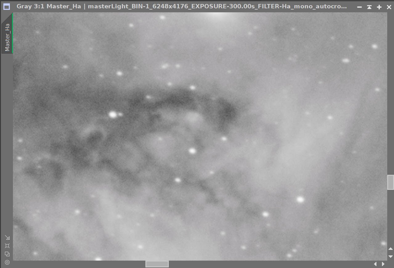
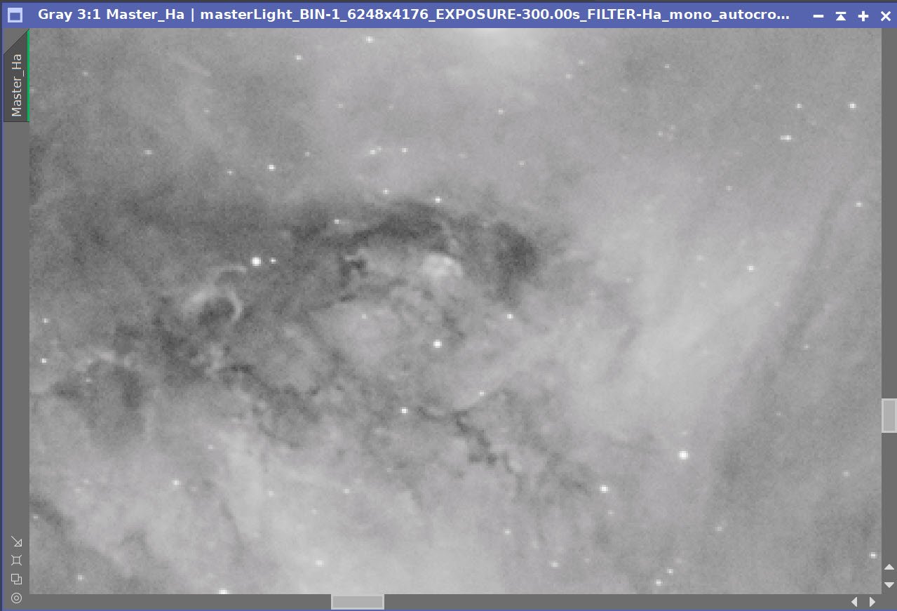
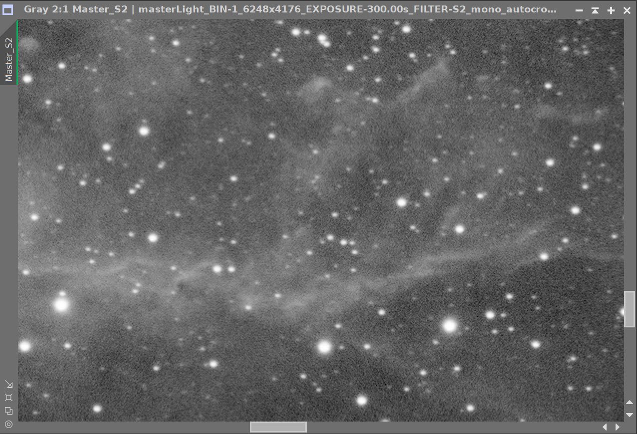
DBE Sample Pattern for Ha Master (click to enlarge)
Before DBE for Ha Master (click to enlarge)
After DBE for Ha Master (click to enlarge)

Background Pattern - Ha Master (click to enlarge)
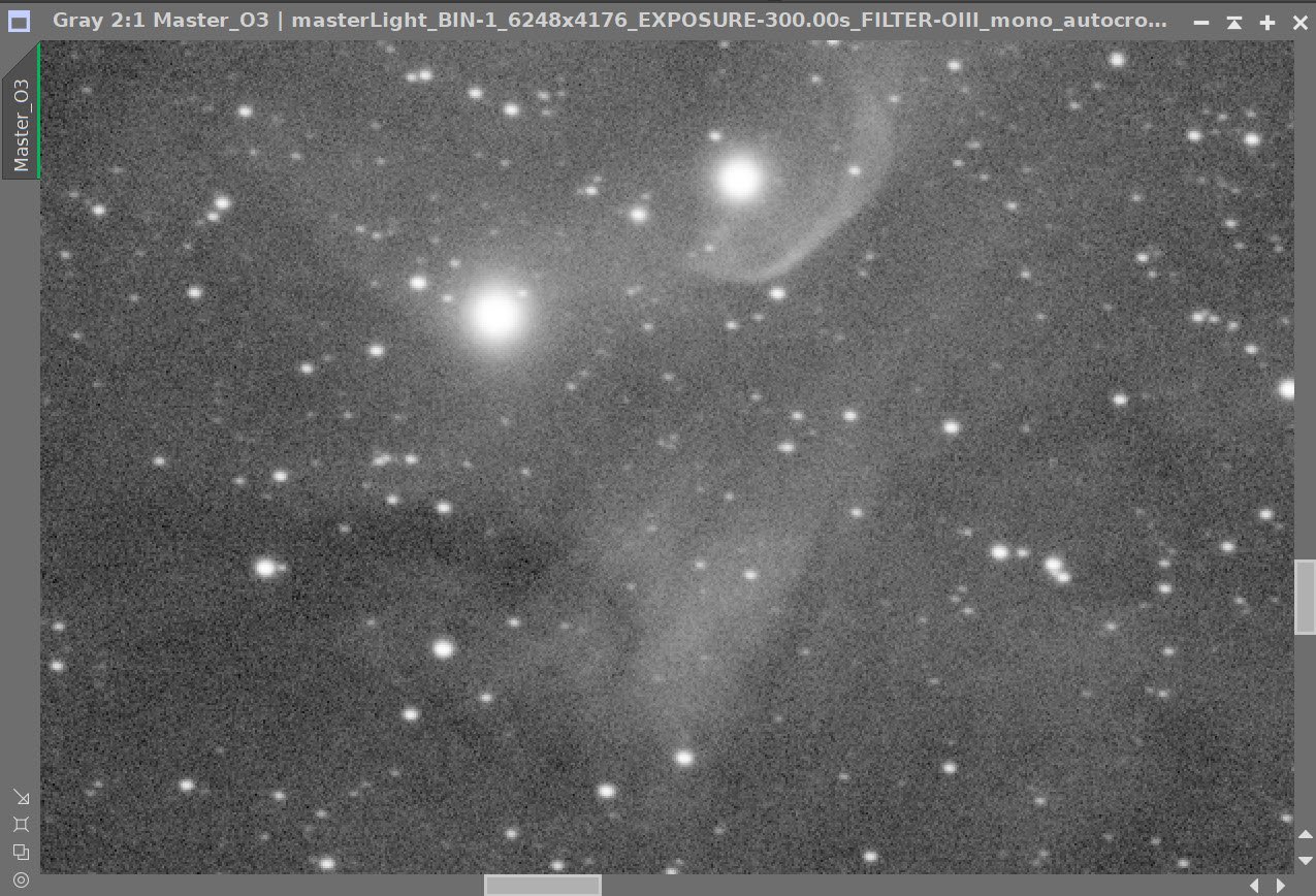
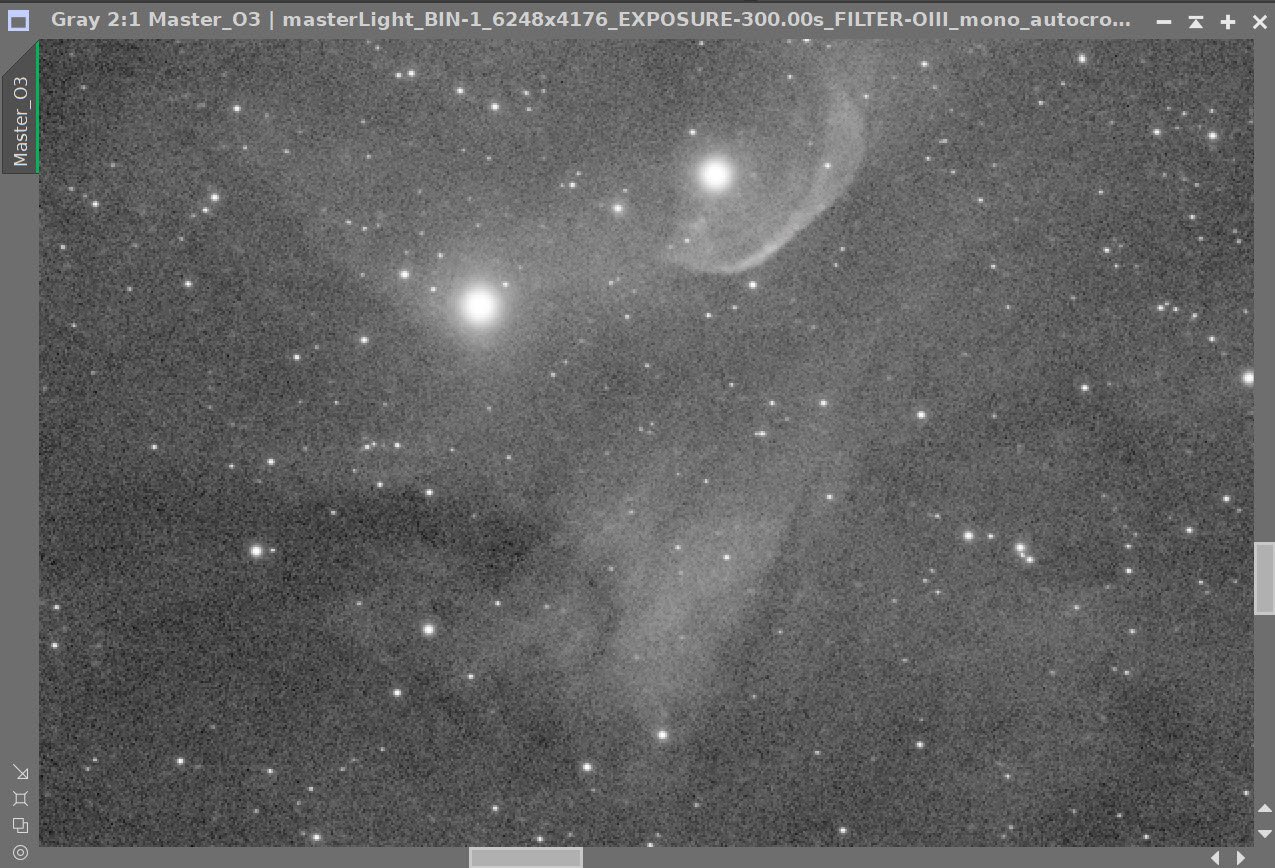
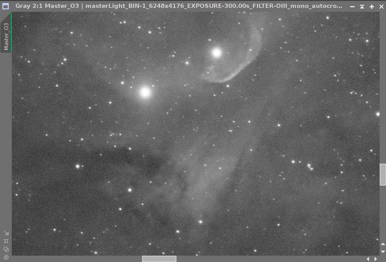
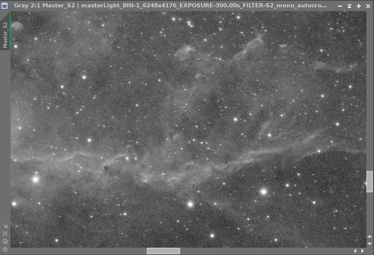
DBE Sample Pattern for O3 Master (click to enlarge)
Before DBE for O3 Master (click to enlarge)
After DBE for O3 Master (click to enlarge)
Background Pattern - O3 Master (click to enlarge)
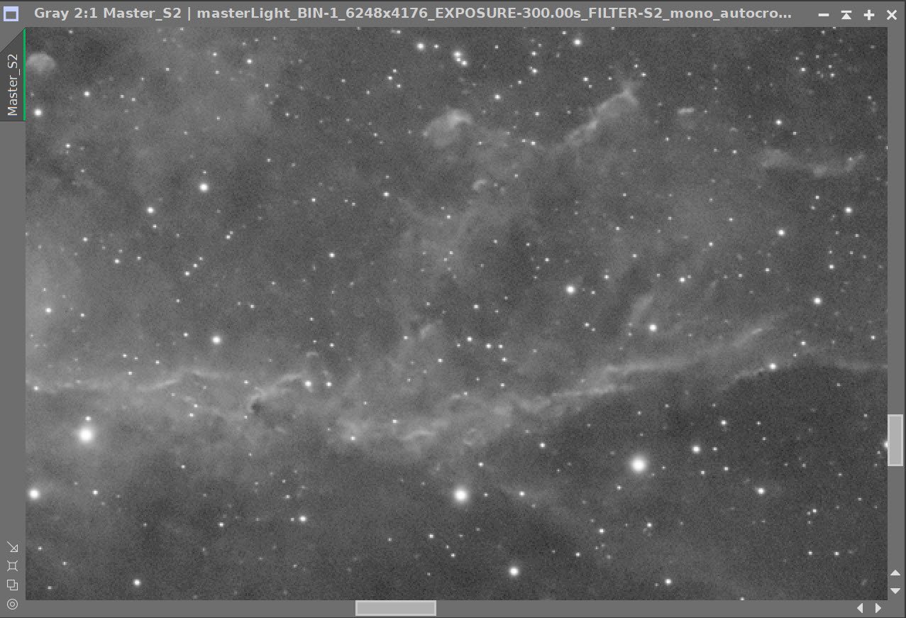
DBE Sample Pattern for S2 Master (click to enlarge)
Before DBE for S2 Master (click to enlarge)
After DBE for S2 Master (click to enlarge)
Background Pattern - S2 Master (click to enlarge)
DBE Sample Pattern for RGB Master (click to enlarge)
Before DBE for RGB Master (click to enlarge)
After DBE for RGB Master (click to enlarge)
Background Pattern - RGB Master (click to enlarge)
5. Complete the Linear Processing of the RGB Image
Do a Color Calibration
Select a preview sample of the background sky
Setup SPCC panel
Run SPCC
Run Deconvolution
Experiment with values - see panel snap for details
Run BXT - see panel snap for details
Run Noise Reduction
Run NXT with a value of 0.65

Starting RGB image - note the preview sample area - along with the setup of the SPCC panel.

SPCC Output with the regression line. Note the strange cluster in the top curve - not sure what is going on there!
Master RGB after SPPC (Click to enlarge)

The BXT Panel Setup for the final run
Master RGB Image Before BXT, After BXT, and after NXT = 0.65
6. Do the Linear Processing for the Ha Image
Run PSFImage to determine star sizes: X=3.36, Y= 2.49
This data set has some guide errors - the stars are somewhat elongated. Fortunately, BXT can correct for much of this when run in Correct First mode. I tend to pick a non-stellar correction PSF size value closer to the smallest or somewhat in between the two values.
Run Deconvolution
Experiment with different values
Run BXT - see panel snap for details
Run Noise Reduction
Run NXT with a value of 0.55

The Output from PSFImage for the Master Ha image.

How the BXT tool was configured for the Master Ha image

The Master Ha Image before BXT, After BXT, and After NXT=0.55
7. Do the Linear Processing for the O3 Image
Run PSFImage to determine star sizes: X=3.24,Y=2.38
Run Deconvolution
Experiment with values
Run BXT - see panel snap for details
Run Noise Reduction
Run NXT with a value of 0.55

Output from PSFImage

BXT Panel set up as run.
The Master O3 Image before BXT, After BXT, and After NXT=0.55
8. Do the Linear Processing for the S2 Image
Run PSFImage to determine star sizes: X=3.2,Y=2.41
Run Deconvolution
Experiment with values
Run BXT - see panel snap for details
Run Noise Reduction
Run NXT with a value of 0.55

Output from PFSImage

BXT Panel as run
The Master O3 Image before BXT, After BXT, and After NXT=0.55
9. Go Nonlinear and Create Starless/Stars-Only Images
For each image
Adjust the STF as needed
Use the STF->HT method to go nonlinear
Remove the stars using StarXTerminator
For Narrowband - run without saving the star images
Run saving the star images for RGB and use the “Unscreen” option.
Create The First color SHO Image:
Use Linfit - with the O3 Starless image as the reference, apply it to the Ha and S2 Starless images. This will reduce the contrast of the other two images down to the contrast of the O3, allowing all to have a more balanced contribution to the image.
Create the first SHO color image using the ChannelCombination process and the S-H-O image sequence.
The initial image is pretty flat - but that’s OK - we will fix that now. Use HT to remove unused areas to the left of the Histogram and balance the peaks of the curves.
Next, we will use CT to boost the contrast - see the CT Panel snapshot below.
This lightens the image - but now we can see a problem! There is a horizontal noise pattern in the data. I am not sure where it came from - maybe its read noise. But we need to fix this!
Run the CanonBandReduction Script and adjust until the bands are no longer evident. For me, a value of about 0.75 did it!
Finally - adjust the Stars Only RGB image to reduce the star intensity and size and boost the saturation using CT.

The initial Ha, O3, and S2 Nonlinear images.

After running StarXTerminator we now have the starless versions

After running Linfit to match the Ha and S2 image to the O3 image.

The initial SHO Starless Image! Very flat - but we will fix that soon!

Red Channel Adjustment

Green Channel Adjustment

Blue Channel Adjustment. Note the 3 color curves are pretty lined up now.

Apply the Histogram Transform to remove unused portion to the left of the histogram and align the peaks.

We will boost the contrast with this CT Adjustment

After boosting the contrast with CT - we can see horizontal noise bands in the image.
Here is the CanonBandReduction Script. The main control is the amount. Greater than one accentuates the bands. Lower than one reduces the bands. I have it set here at about 3.0 so you better see the subtle bands I was seeing. (click to enlarge)
In this image, I have reduced the Amount to 0.75 and to my eye, that eliminated the problem nicely! (click to enlarge)

After running the CanonBandReduction Script, the problem is no longer detectable!

Here is our initial nonlinear RGB image.

And here is the Stars-ONLY image after Running StarXTerminator.

We finish up our processing of our Stars Only image but adjusting with CT to reduce the star intensity and size, and boosting the color saturation just a tad.

Here is the Curves Adjustment we made. Top curve is Saturation. The bottom is RGB/K.
10. Do the Initial Color Processing on the SHO Starless Image
Run SCNR with Green Removal at 0.85
Invert the image. What was magenta is now green!
Run SCNR with Green Removal at 0.85 again.
Invert the Image
Now do a global boost for both contrast and color saturation.
The Starting Point (click to enlarge)

After Inverting the Image. What was magenta is now green! (click to enlarge)
After a final Invert (click to enlarge)
After SCNR Green - with an amount of 0.85 (click to enlarge)
After SCNR Green - with an amount of 0.85 (click to enlarge) - thus removing any residual magenta.

After a final CT adjustment (click to enlarge)
11. Create the Color Masks We Will Need to Adjust Our Image
Create the Blue Color Mask
Run Bill Blanshan Blue Color Mask Script
Use CT to boost the Contrast
Create the Green Color Mask
Run Bill Blanshan Green Color Mask Script
Use CT to boost the Contrast
Create the Yellow Color Mask
Run Bill Blanshan Yellow Color Mask Script
Use CT to boost the Contrast
Apply Bill Blansan Blur
Use CT to do another boost the Contrast
Apply ANotehr Bill Blansan Blur
Create a BOW_Wave Mask
Use GAME to create a gradient ellipse that covers the bow wave of Cygnus X-1
Initial Blue Mask from the Bill Blanshan Script (click to enlarge)
Initial Green Mask from the Bill Blanshan Script (click to enlarge)
Initial Yellow Mask from the Bill Blanshan Script (click to enlarge)
Yellow Mask After the Bill Blanshan Blur Script (click to enlarge)
Yellow Mask - after final Blur (Click to enlarge)
The same mask after CT adjust (click to enlarge)
The same mask after CT adjust (click to enlarge)
The same mask after CT adjust (click to enlarge)
The same mask after ANOTHER CT adjust (click to enlarge)
The GAME Mask designed to cover the region with the Cygnus X-1 Shock wave (click to enlarge)
12. Do Initial Mask Processing
Apply the Green Mask - this often is associated with the “Golden” portions of the SHO palette.
Adjust with CT
Enhance the details in this area using Local HistgramEqualization (LHE) with a 64-pixel radius, 2.0 contrast limit of 0.25 amount and an 8-bit histogram
Apply the Blue Mask
Adjust with CT
Enhance the details in this area using Local HistgramEqualization (LHE) with a 64-pixel radius, 2.0 contrast limit of 0.50 amount and an 8-bit histogram
The starting point.(click to enlarge)
With Green Mask Applied, a CT adjust has been done (click to enlarge)
After LHE applied to the Green Masked areas (click to enlarge)
After LHE with the Blue Mask (click to enlarge)
CT adjust with the Blue Mask (click to enlarge)
13. Create a Dark Structure Mask and Use It
At this point, I decided I wanted to work on the Dark Structures. Rather than just using the DarkStructureEnhance Script, I like to use it to create the mask - which I then manipulate.
Create the Mask
Run the DarkStructureEnhance script with all defaults and check the ‘extract mask’ option.
Enhance the Mask with a CT adjustment.
Blur with BB Blur Tool
Do a final CT
Apply the Mask
I experimented with making a CT adjustment but decided using this mask to make some selective contrast sharpening with LHE would be better.
Enhance the details in this area using Local HistgramEqualization (LHE) with a 16-pixel radius, 2.0 contrast limit of 0.66 amount, and an 8-bit histogram.
Mask returned from DSE (DarkStructuresEnhance) (click to enlarge)
After Blurring with the Bill Blanshan tool. (click to enlarge)
Before the Dark Mask LHE Operation (click to enlarge)
Mask adjusted with CT (click to enlarge)
Dark Mask after final CT (Click to enlarge)
After LHE with the Dark Mask (click to enlarge)
14. Final Tweaks to the Starless Image
Apply NXT with a value of 0.65 to the image
Do a CT global adjust
Apply The GAME Mask to the image to focus on the bow wave area
Enhance the details in this area using Local HistgramEqualization (LHE) with a 50-pixel radius, 2.0 contrast limit= 0.40 amount, and an 8-bit histogram.
Apply the Yellow Mask
Enhance the details in this area using Local HistgramEqualization (LHE) with a 38-pixel radius, 2.0 contrast limit= 0.20 amount, and an 8-bit histogram.

Before and After NXT=0.55
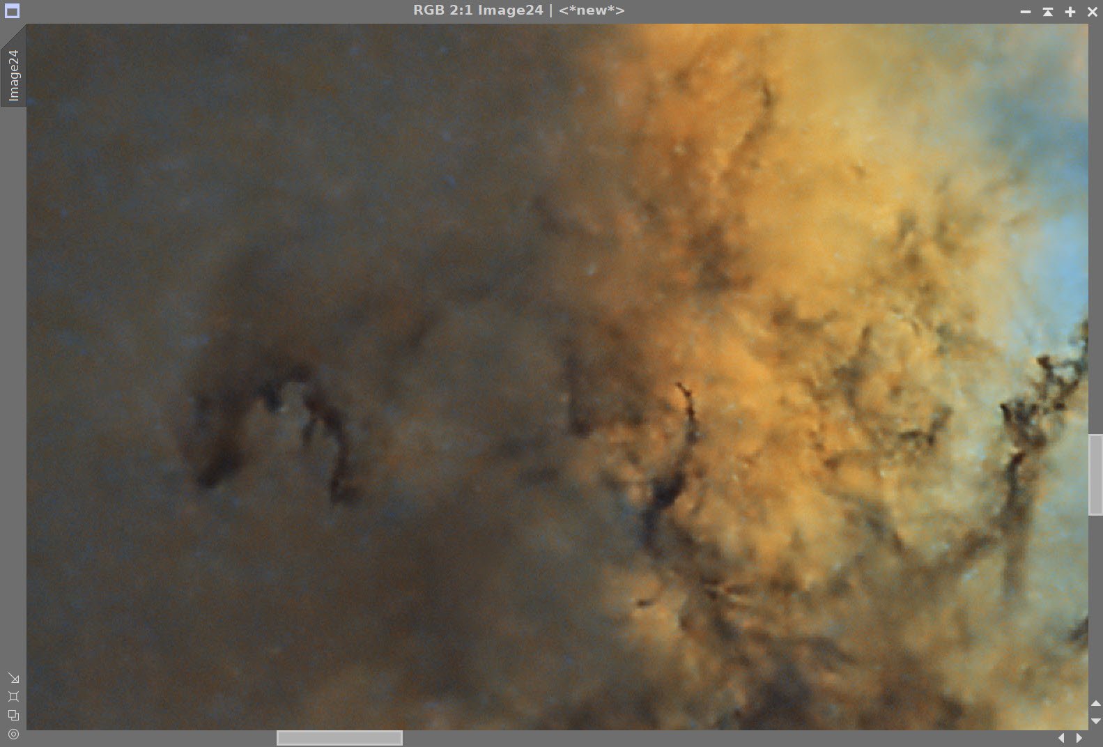
Before Bow Shock Wave LHE application (click to enlarge)
After Bow Shock Wave LHE application (click to enlarge)

The Final Starless Image after the LHE operation with the Yellow Mask
15. Add the Stars Back in!
Using PixelMath and a screening equation (see screen snap) - create a new image with the Stars added back in

The screening equation used to add the stars back in.

The first images with the Stars added back in!
16. Export the Image to Photoshop for Polishing
Save the image as Tiff 16-bit unsigned and move to Photoshop
Adjust with Clarify and Color Mixer
Do a final curves
Add water marks
Export Clear, Watermarked, and Web-sized jpegs.

The Final Image!
Adding the next generation ZWO ASI2600MM-Pro camera and ZWO EFW 7x36 II EFW to the platform…