
NGC 6888 - A Reprocess of The Crescent Nebula ~11 hours in HOOrgb
Date: July 7, 2023
Cosgrove’s Cosmos Catalog ➤#0124

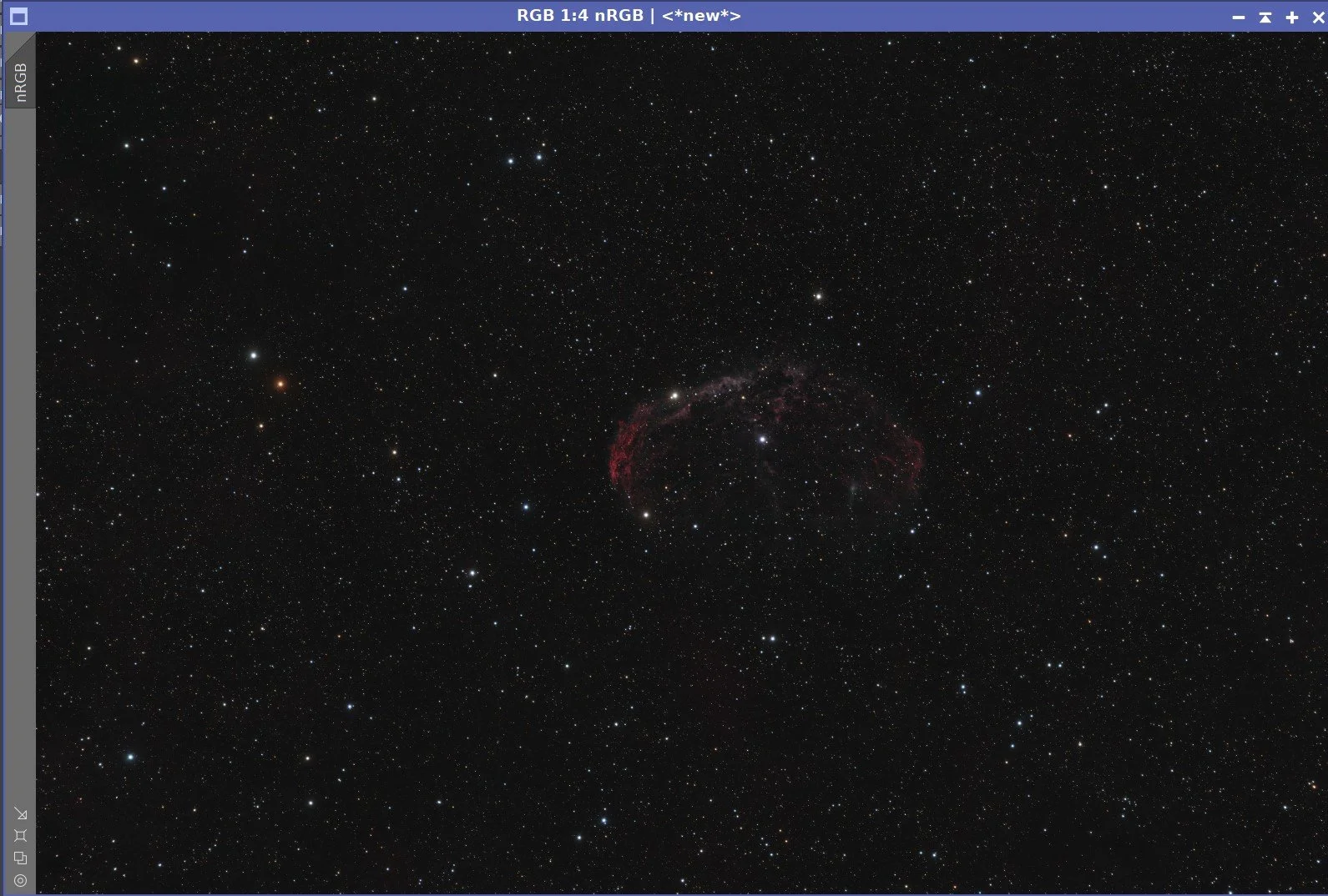
My Reprocess of my NGC 6888 - the Crescent Nebula - in Bi-color - HOO - with RGB stars. The goal of this effort was to enhance the O3 signal and bring more detail to the cyan shell around the nebula (click on the image for a full res version via Astrobin.com)
Awarded Flickr Explore Status on July 8, 2023!

Table of Contents Show (Click on lines to navigate)
About the Target
NGC 6888 - The Crescent Nebula - is an emission nebula located about 5000 light-years away in the constellation of Cygnus. It is also known as Caldwell 27 and Sharpless 105.
This object can be seen visually with a modest telescope, which appears as a crescent shape - thus its name. This view can be improved by using a UHC or O-III filter.

Friedrich Wilhelm Herschel (1738-1822). Image taken from Wikipedia.
This object was discovered and cataloged by William Herschel in 1792.
Wikipedia describes it thusly:
It is formed by the fast stellar wind from the Wolf-Rayet star WR 136 (HD 192163) colliding with and energizing the slower moving wind ejected by the star when it became a red giant around 250,000 to 400,000 years ago. The result of the collision is a shell and two shock waves, one moving outward and one moving inward. The inward-moving shock wave heats the stellar wind to X-ray-emitting temperatures.
The Annotated Image

This annotated image was created using the Pixinsight ImageSolve and ImageAnnotation scripts.
The Location in the Sky

This finger chart was created in Pixinsight using the FinderChart process.
About the Project
Revisiting Some Good Data
2023 is turning out to be a disappointing year for Astrophotography.
First, I had a late start due to my recovery from some surgery. Then wildfires in Canada (first in Alberta and Later in Quebec and Nova Scotia) had blanketed our skies in a way that we had never experienced before - with Air Quality Alerts, Yellow, foggy days that smelled of smoke, and skies that were unsuitable for astrophotography.
This may last for the better part of a year! In the worse case, it may be the new normal.
So to keep busy, I have been revisiting some old data and applying new tools and methods to see where I could take the final results.
I first did this with my Messier 27 image and was surprised at how much more detail I could bring out. The resulting image was selected as NASA’s APOD for May 30th, was published in the September Issue of Sky & Telescope, and will be the Image of the Month for August in BBC’s Sky @ Night Magazine! So the effort has certainly paid off!
Now I am l looking to do the same for the data collected for my NGC 6888 image.
Many astrophotographers have shown the cyan outer shell of O3 gas surrounding the core of the nebula - my previous image also showed this as well. But I wondered if I could bring out even more detail.
So I set that as my goal.
How much further could I take this image using new tools and methods?
Previous Efforts
So what could/Should I do differently this time around?
In the last effort, I created a synthetic Luminance image and used a Lum vs. Color processing workflow.
The resulting workflow can be seen below in a high-level view:

The process flow used in my original processing effort.
So, why did I do it this way?
At that point, I was using the traditional Deconvolution methodology. I found this so painful that I adopted the Lum vs. Color processing path to minimize my efforts there. The idea was to emphasize color position and low noise when processing the color image and then emphasize detail and sharpness in the Lum processing. That way, I only had to do deconvolution on the single Lum image. The final image would inherit the benefits of this sharpness restoration when I used LRGBCombination to fold the Lum and the Color Images back together.
This kind of processing is pretty common.
But to pull it off, I needed to have a Lum image - which I did not have as this was a narrowband HOO image.
So I created a Synthetic Lum image! If this were a full SHO image with Ha, O3, and S2 contributions, I would have created this using the ImageIntegration process to weigh the input images on their SNR contributions to create a new Lum image.
But in this case, my primary data consisted only of Ha and O3 filter information. ImageIntegration required at least three input images - so I could not use that.
So I used a weighted combination of the Ha and O3 image. I experimented with different weights and found that a 50-50 mix of Ha and O3 did best. So I used this to create a Synthetic Luminance image and then did deconvolution on that image.
Reflecting back on it, I realized this approach has a problem.
Since the Lum image was a blend, I was not getting the best sharpness restoration from Deconvolution for each channel. I got one for a channel that diluted the contributions of each filter. For a lot of images, I don’t think that this would be a big problem. But I think it ultimately was not the best approach for this one.
A New Approach
If I ran deconvolution on the Ha and O3 images, I might achieve better detail for each.
So I wanted to try that this time around.
I now also use BlurXTerminator - a wonderful tool that dramatically outperforms traditional deconvolution. I also wanted to use this and see how much it could help.
It usually is best to run BlurXTerminator (herein called BXT) on color images, as it will optimize results between the three layers. This helps to ensure that you get the best stars in your image. If you run BXT on the separated mono image, it cannot do this optimization. You risk having stars coming out with different sizes for each channel and ending up with color rings around them. But I am not worried about the problem here, as I planned to remove the narrowband stars and replace them with RGB stars. So the stars for these images will not be a factor.
Also, note that I am running BXT on the RGB color images, so my color stars - which I will be using - should be well-optimized!
Another issue is how I did the starless processing the last time around. I was using StarNet2 for removing stars. Now I own StarXTermintor (Herein called STX), which does a much better job.
With this in mind, my workflow would change to something that looks like this:

My new proposed workflow for this processing run.
Image Processing
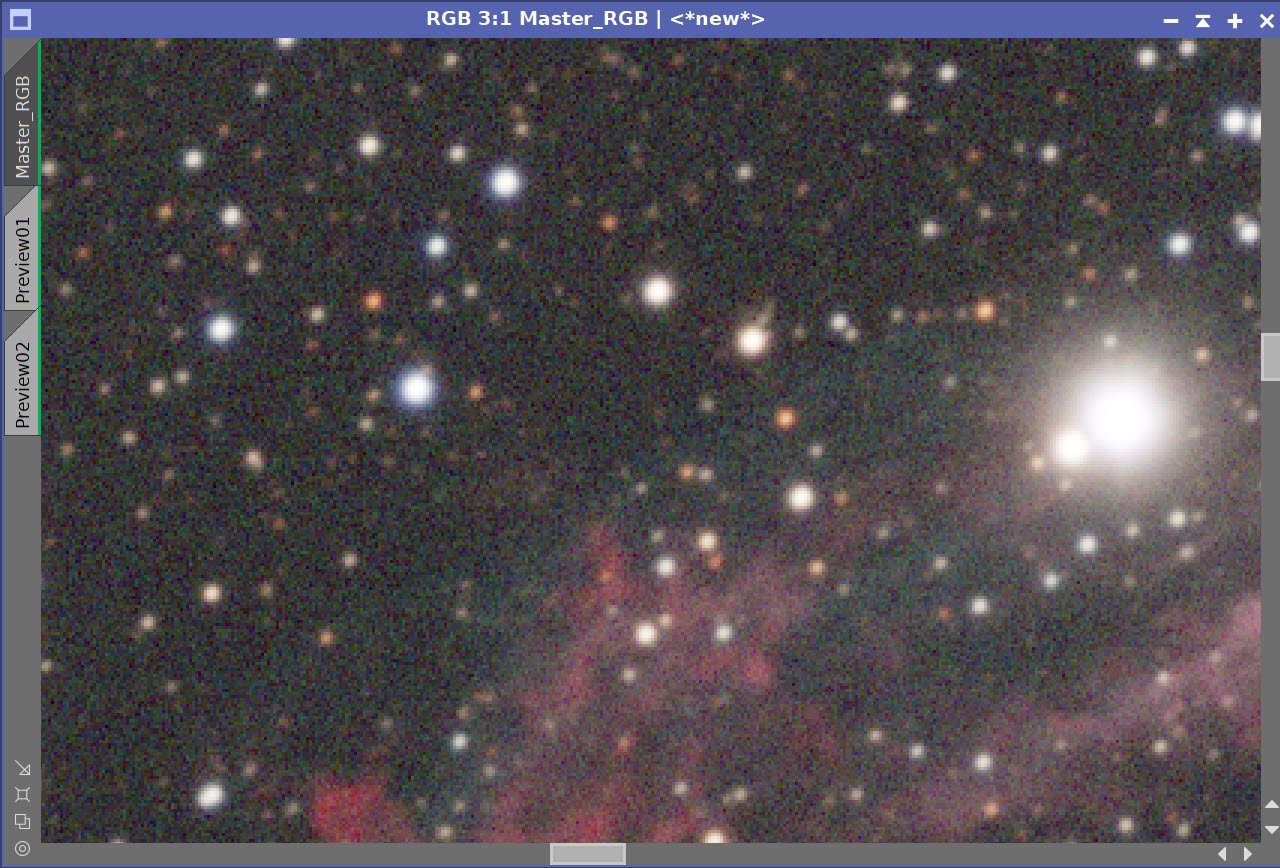
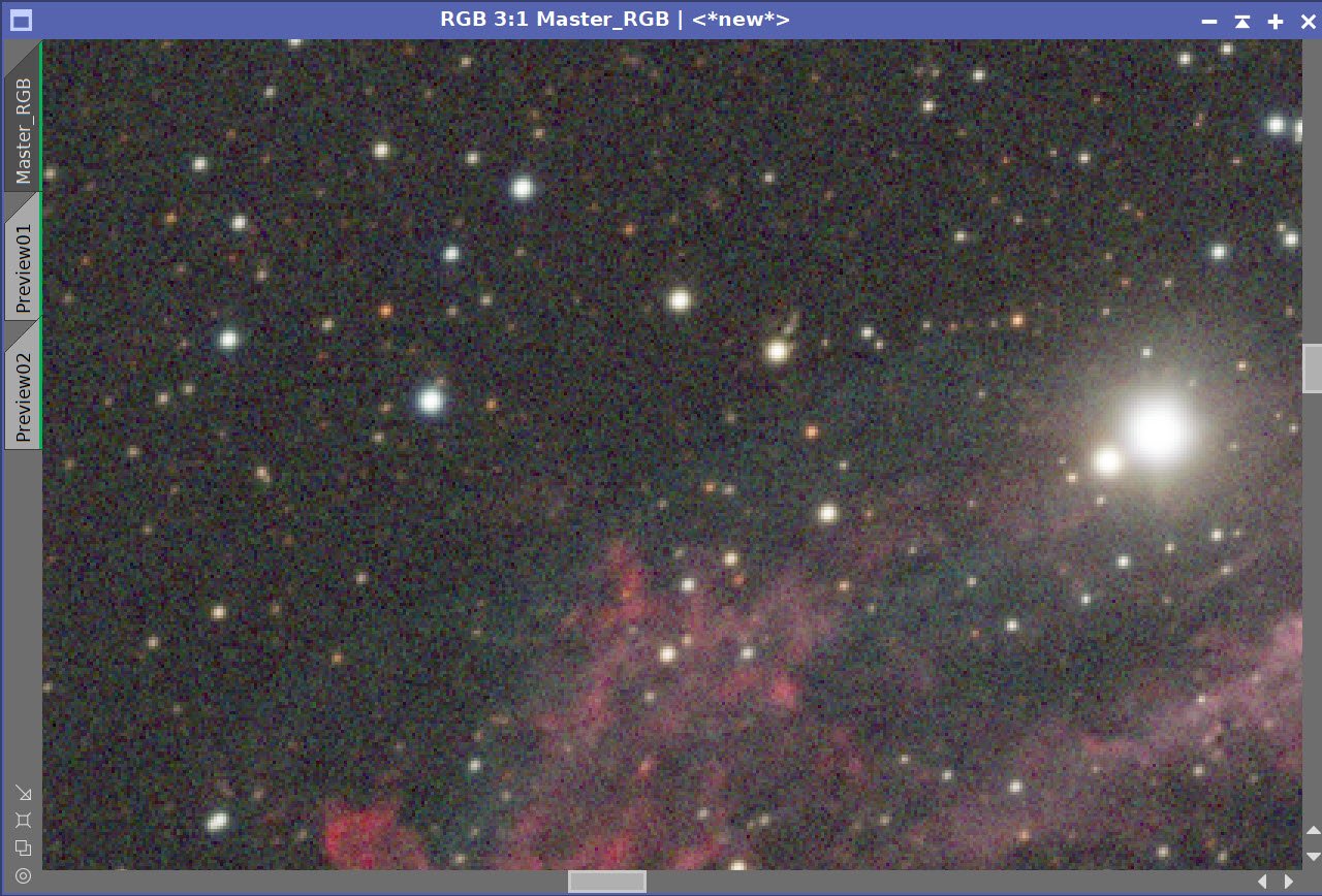
The image processing went fairly smoothly. Following my proposed approach, I was finding the improvements I had hoped for. I could see more structure and detail in the resulting O3 image. When I created the HOO image, I found that the O3 detail was much more evident. However, as the O3 detail seemed to pop, it did seem to come at the expense of some Ha detail and color. This produced an initial new image comparison that you can see below:
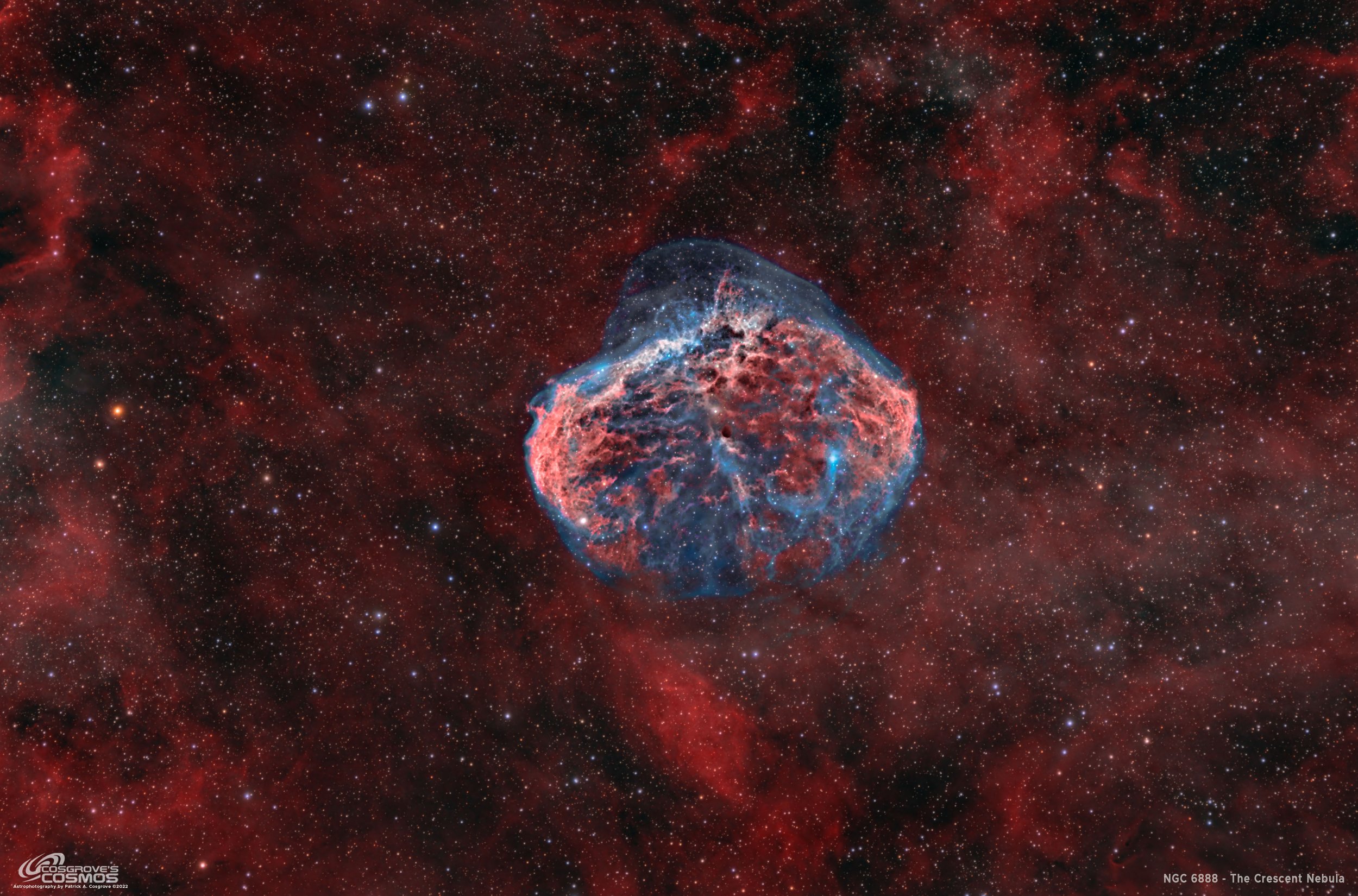
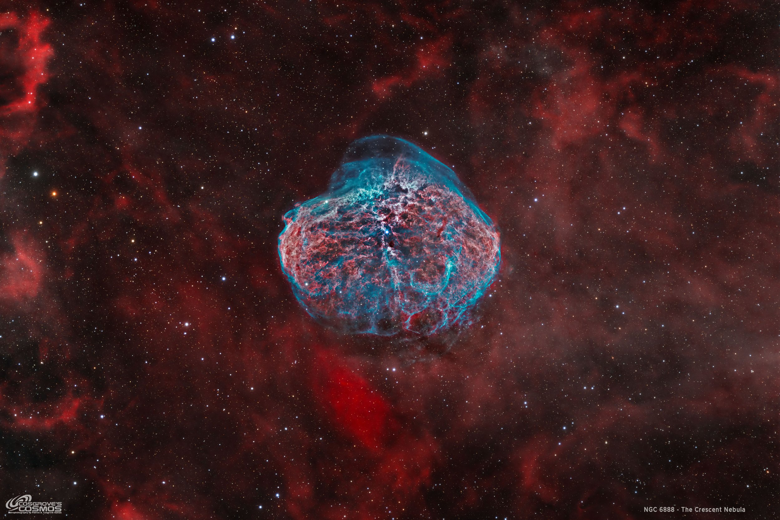
The original image (click to enlarge)
The first cut at a Reprocessed image (click to enlarge)
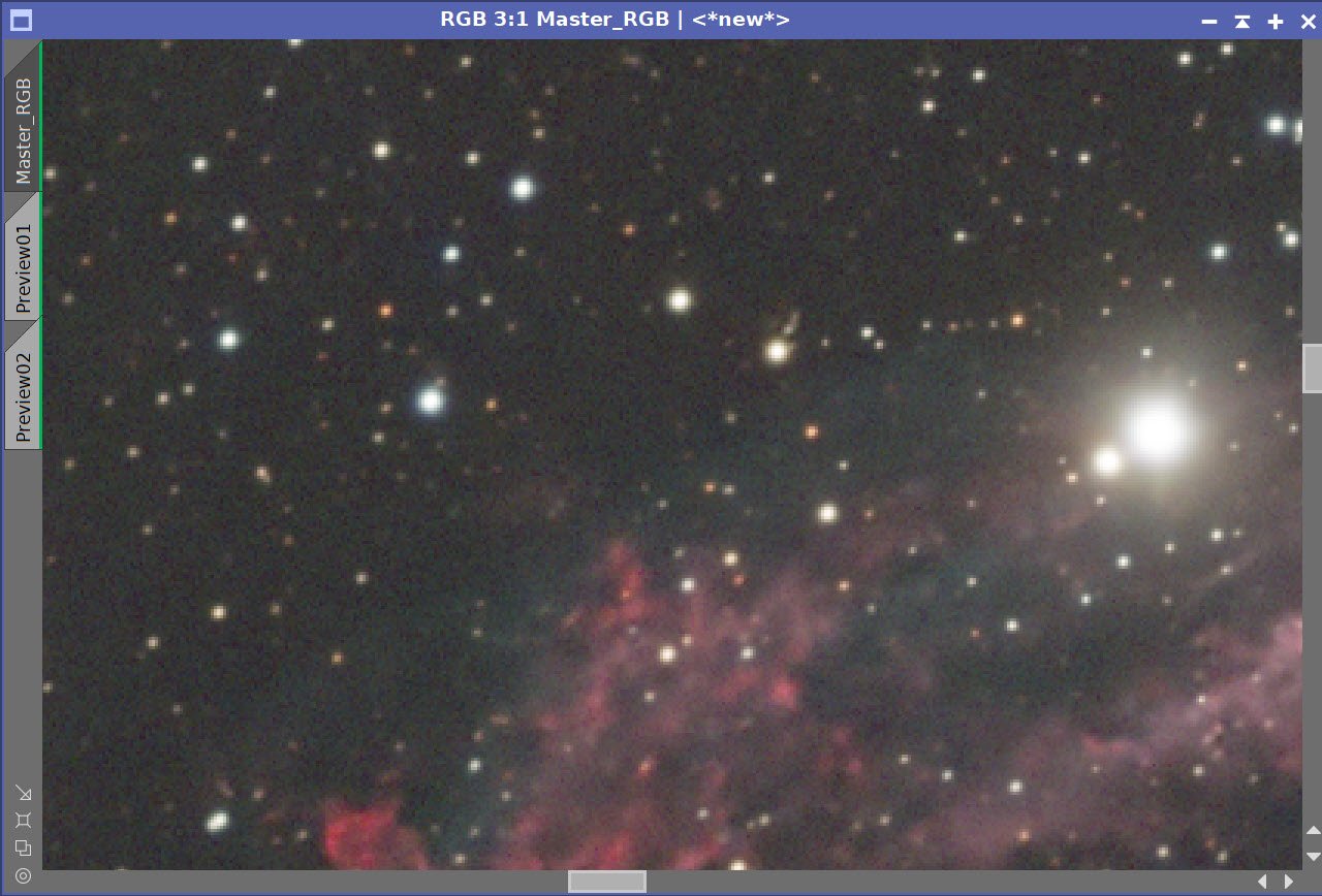
I liked this version, but I missed the brighter orange-red color in the main body of the nebula where the Ha signal dominates. The core of the nebula looked a little drab. I decided to try and create a special Red-Mask that would specifically target the Ha structure in the body of the nebula and adjust its color in a tightly focused effort. If I went too far, I might lose some of the O3 detail I fought to gain. This produced my final image, which can be seen below. It is a modest improvement, but I think I restored some lost color without swamping the O3 improvements.
The final image brings up the color slightly in the core of the nebula.
Image Results
I am pretty happy with the results of this effort.
Stars: BXT created nice, tight, and well-formed stars. STX did a much better job of removing the stars and the screening method of adding stars back in produced a very natural result. In fact, If you look carefully, you see some stars in the older image that are just plain missing - whereas this is not a problem in the new image.
Ha Details: To an extent, I did trade off Ha details to highlight the O3 details. But I don’t think it hurt the Ha that much. Clearly, the Ha was the dominant signal, but I could bring the O3 detail up without a severe degradation to the Ha.
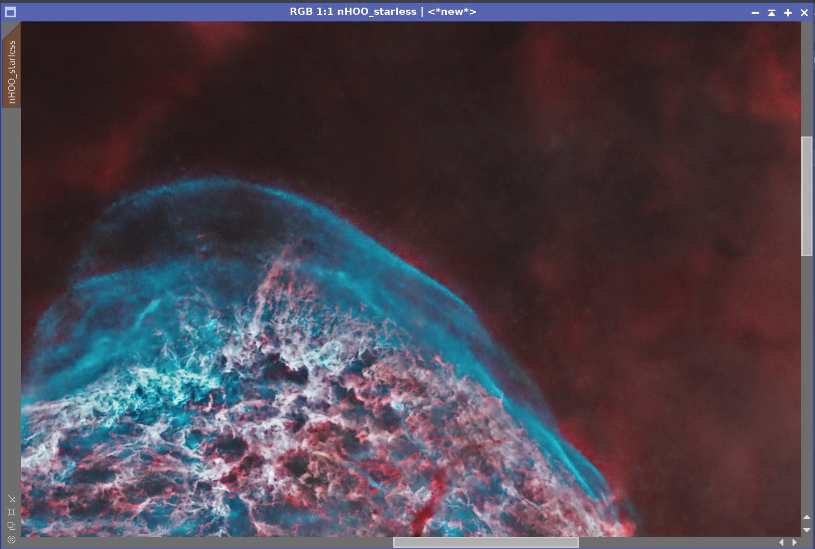
O3 Details: I am super happy with where the O3 details are now. The upper plume has a lot more complexity, and towards the bottom of the nebula, you can see a cellular structure in the gas that is just fascinating. Furthermore, you can see very faint gas extensions off the bottom of the nebula. I have not seen that many images of NGC 6888 that show this kind of detail, so I am happy with the results!

The Old Version Vs. The New
A detailed Processing Walk-Through is provided for this image at the end of the posting…
Capture Details
Lights Frames
Data was collected over four nights: Aug 24, Aug 28, Sept 1, and Sept 2
Number of subs after Blink and removal
85 x 300 seconds, bin 1x1 @ -15C, Gain 100, Astrodon 5nm Ha
39 x 300 seconds, bin 1x1 @ -15C, Gain 100, Astrodon 5nm O3
10 x 90 seconds, bin 1x1 @ -15C, Gain 100, ZWO gen 2 Red
10 x 90 seconds, bin 1x1 @ -15C, Gain 100, ZWO gen 2 Green
10 x 90 seconds, bin 1x1 @ -15C, Gain 100, ZWO gen 2 Blue
Total of 11 hours and 5 minutes
Cal Frames
25 Darks at 300 seconds, bin 1x1, -15C, gain 100
30 darks at 90 seconds bin 1x1, -15C, gain 100
12 Flats at bin 1x1, -15C, gain 100 - for Ha, O3, R, G & ,B filters
25 Dark Flats at Flat exposure times, bin 1x1, -15C, gain 100
Software
Capture Software: PHD2 Guider, Sequence Generator Pro controller
Image Processing: Pixinsight, Photoshop - assisted by Coffee, extensive processing indecision and second-guessing, editor regret, and much swearing…..
Capture Hardware:
Scope: Astro-Physics 130mm F/8.35 Starfire APO built in 2003
Guide Scope: Televue TV76 F/6.3 480mm APO Doublet
Main Fous: Pegasus Astro Focus Cube 2
Guide Fous: Pegasus Astro Focus Cube 2
Mount: IOptron CEM60 - new
Tripod: IOptron Tri-Pier with column extension - new
Main Camera: ZWO ASI2600MM-Pro - new
Filter Wheel: ZWO EFW 7x36 - new
Filters: ZWO 36mm unmounted Gen II LRGB filters - new
Astronomiks 36mm unmounted 6nm Ha,
OIII, & SII filters - new
Rotator: Pegasus Astro Falcon Camera Rotator
Guide Camera: ZWO ASI290MM-Mini
Power Dist: Pegasus Astro Pocket Powerbox
USB Dist: Startech 7 slot USB 3.0 Hub
Software:
Capture Software: PHD2 Guider, Sequence Generator Pro controller
Image Processing: Pixinsight, Photoshop - assisted by Coffee, extensive processing indecision and second-guessing, editor regret and much swearing…..
Click below to see the Telescope Platform version used for this image:
Image Processing Walk-Through
(All Processing is done in Pixinsight - with some final touches done in Photoshop)
1. Blink Screening Process (same as old processing)
Ha
Some gradients
A few trails
No frames eliminated
O3
Lots of thin clouds attenuating the signal
11 frames removed!
Red
all fine
Green
all fine
Blue
some faint trails but otherwise, all fine
Flats
Collected on night two only. Data looks good
RGB collected on night 4 - all ok.
Dark flats
Ha and O3 were collected on the second night - data looks good
RGB collected on night 4 - all ok.
2. WBPP 2.5.0
First use of version 2.5.0 - still not yet familiar with its new features.
Reset everything
Load all lights
Load all flats
Load all darks
300-sec from 7-26-22 cal data
I did not have 90- darks with gain 100, so I used gain zero darks from 7-26-22. Since this is just for stars, I figured I could get away with it.!
Select - maximum quality
Reg reference - auto - the default
Select output directory to wbpp folder
Enable CC for all light frames
Pedestal value - auto for NB filters
Darks -set exposure tolerance to 0
Lights - set exposure tolerance to 0
select integration mode - just cal and alignment
Map flats and darks across nights
Set autocrop
Executed in 1:15

WBPP Calibration view.

WBPP Post-Calibration View.

WBPP Pipeline View
3. Load Master Images
Load all master images and rename them.
Rotate all images 180 degrees (so the image looks right-side up to my eyes)
Create the RGB Master Image by using ChannelCombination

Initial Master Ha and O2 linear images!

Initial Master Red, Green, and Blue linear images!

Master narrowband images after rotation.

Master R,G, and B images after rotation.
The Initial RGB Master Image.
4. Dynamic Background Extraction
DBE was run for each image using the subtraction method. Below are the Sampling plans, the before image, the after image, and the removed background images.
DBE: Ha Sampling (Click to enlarge)
Ha image Before DBE (click to enlarge)
Ha image After DBE (click to enlarge)
Ha background removed (click to enlarge)
DBE: O3 Image Sampling (Click to enlarge)
O3 Image Before DBE (click to enlarge)
O3 Image After DBE (click to enlarge)
O3 background removed (click to enlarge)
DBE: RGB Sampling (Click to enlarge)
RGB image Before DBE (click to enlarge)
RGB Image After DBE (click to enlarge)
RGB background removed (click to enlarge)
5. Finish the Linear Processing on the Narrowband Master Images
For the Master Ha Image:
Run the PSFImage Script to get a measure of star sizes.
FWHM X = 2.95
FWHM Y = 3.44
Test and experiment with different BXT values.
Pick the Final Value and Run BXT
See the screen snap of the BXT Panel to see the values used.
Run NXT at 0.55
For the Master O3 Image:
Run the PSFImage Script to get a measure of star sizes.
FWHM X = 2.86
FWHM Y = 3.44
Test and experiment with different BXT values.
Pick the Final Value and Run BXT
See the screen snap of the BXT Panel to see the values used.
Run NXT at 0.55
Master Ha Processing

The star size seems to be about 3.0 - once corrected.

Here is how I ran the Ha BXT - the stellar adjustments are default as I will be removing the stars later and discarding them. I am running “Correct First” mode, and using a manual Nonstellar Sharpening of 3.0
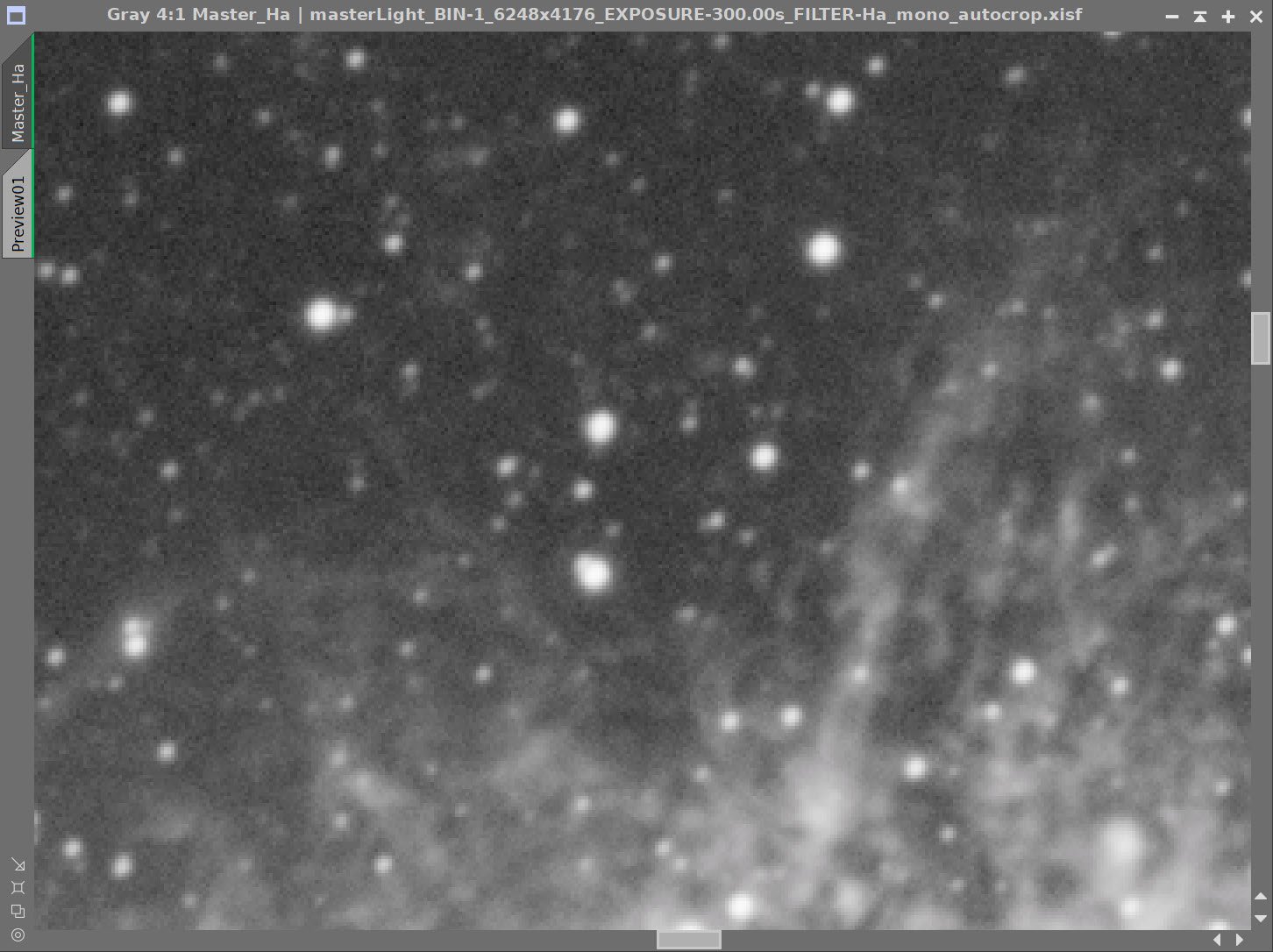

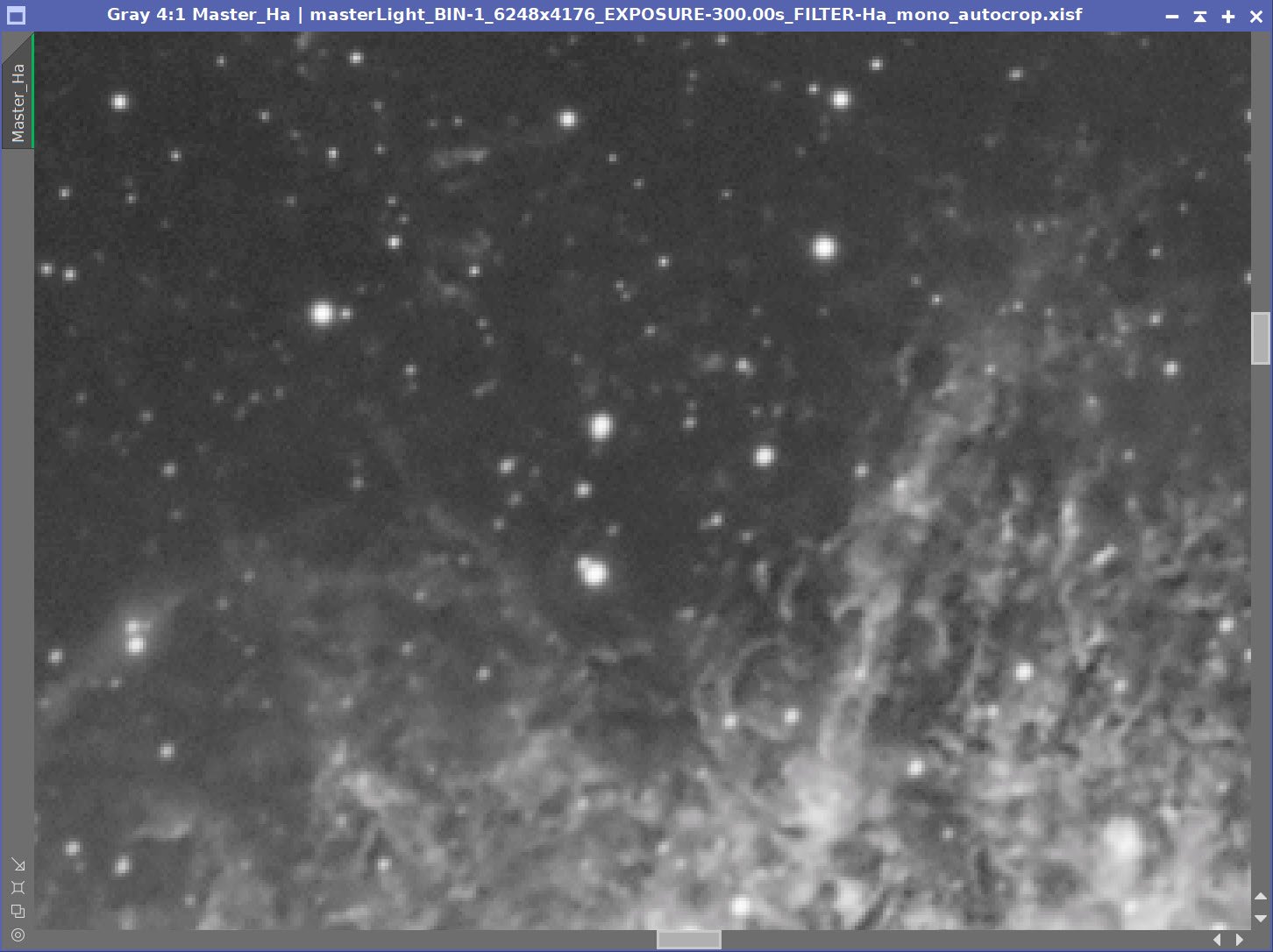
Master Linear Ha Image - Before and After BXT and NXT 0.55
Master O3 Processing

The star size seems to be about 2.85 - once corrected.
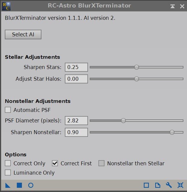
Similar to the Ha BXT - the O3 is run with the stellar adjustments are default asI on’t care about them . I am running “Correct First” mode, and using a manual Nonstellar Sharpening of 2.82 - it should have been 2.85 but I had a typo! Close enough!
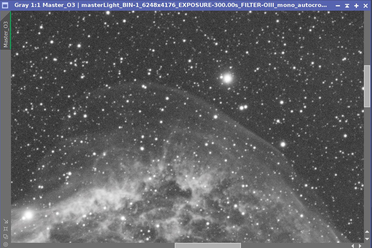
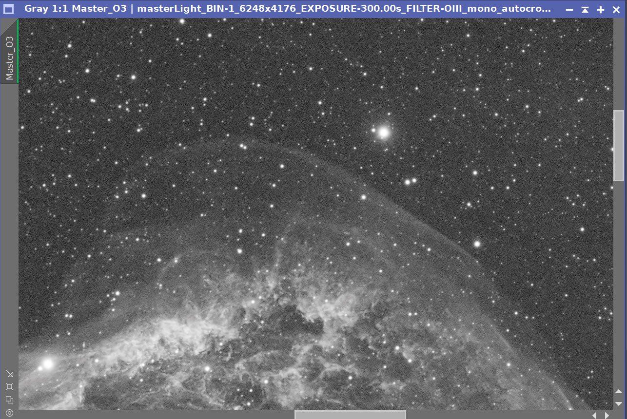
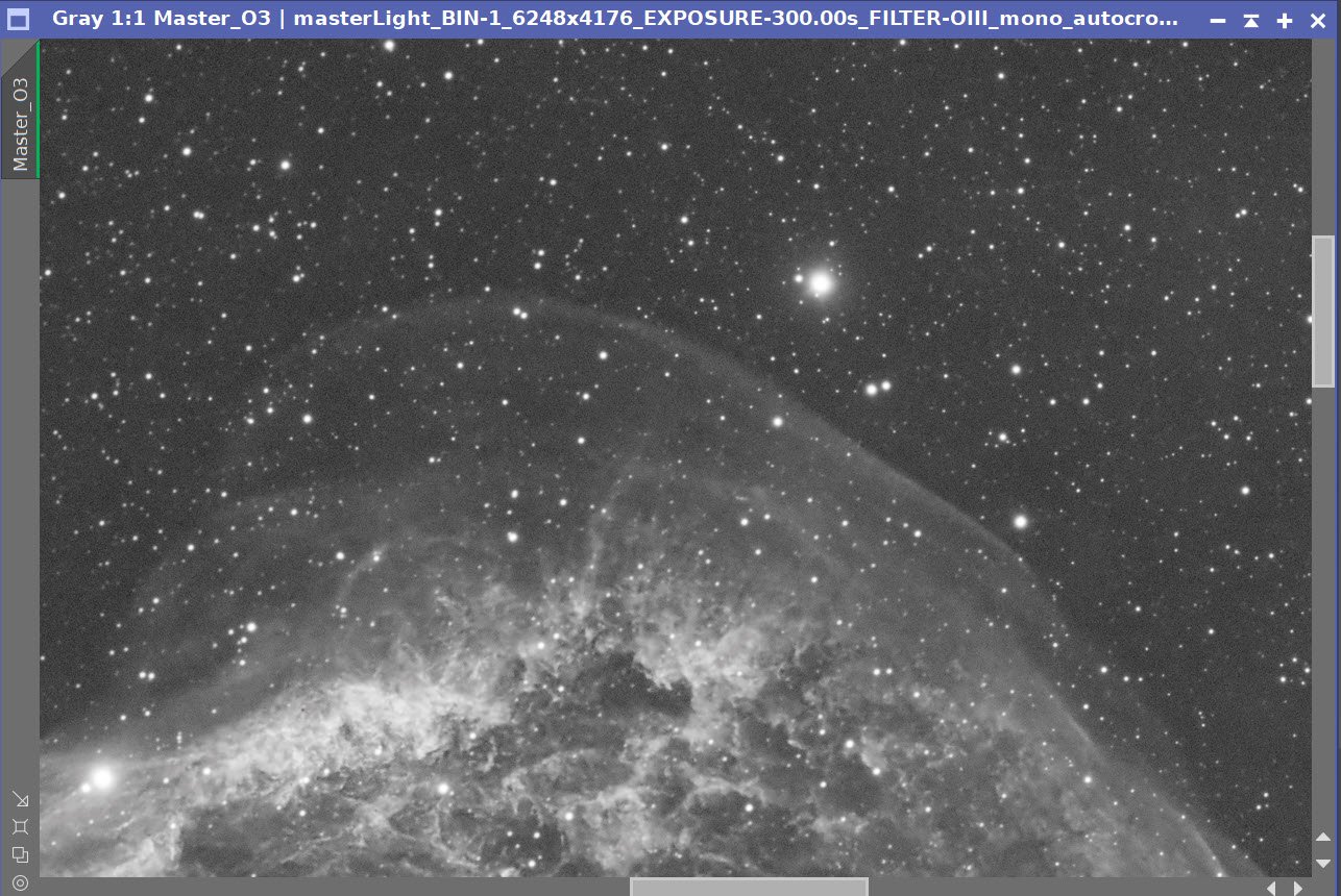
Master Linear O3 Image - Before and After BXT and NXT 0.55
6. Finish the Linear Processing on the RGB Master Images
For the Master RGB Image:
Run the ImageSolver script to get a new astrometric solution. Our crop and rotate messed up the one that was placed there by WBPP. Pixinsight should handle this automatically when crops and rotates are done, but right now, it does not. We will need this data in the image to run SPCC
Run SPCC, setting the right filter types and sensor type (see screen snap below)
Run the PSFImage Script to get an idea about star size.
FWHM X = 2.86
FWHM Y = 3.44
Test and experiment with different BXT values.
Pick the Final Value and Run BXT
See the screen snap of BXT Panel to see the values used.
Run NXT at 0.65 (a little more aggressive than what I used on the narrowband images.

SPCC Parameters used

Regression Line reported by SPCC
Master RGB Before SPCC (click to enlarge)
Master RGB After SPCC (click to enlarge)

The star size seems to be about 2.53 - once corrected. The stars are smaller - which is great. That will be much tighter than the narrowband stars. This is now to know, but I will not use these star sizes in BXT.

Here is how I ran the RGB BXT - a little more aggressive on the Star Sharpening side, but I just ran the nonstellar at the defaults I was not going to use the nonstellar data. .
Master Linear RGB Image - Before and After BXT and NXT 0.65
7. Go Nonlinear and Starless with the RGB and Narrowband images
Go Nonlinear and Starless for RGB
Copy the Master RGB image and rename: “nRGB”
Adjust the STF mapping to get the stars you like
Use the STF->HT method to go Nonlinear
Copy the image and rename it to “nRGB_Starless”
Run STX: Create Star Images and use Screening.
Run CT on the stars image to reduce the intensity and boost saturation a bit
Go Nonlinear and Starless for Ha
Copy the Master Ha image and rename: “nHa”
Adjust the STF mapping to get the image you like
Use the STF->HT method to go Nonlinear
Copy the image and rename it to “nHa_Starless”
Run STX: Do not create star images
Go Nonlinear and Starless for O3
Copy the Master O3 image and rename: “nO3”
Adjust the STF mapping to get the image you like
Use the STF->HT method to go Nonlinear
The O3 image seems a little lighter so adjust with HT
Copy the image and rename it to “nO3_starless”
Run STX: Do not create star images
Nonlinear and Starless RGB Images
Nonlinear RGB Image (click to enlarge)
Initial Stars Only Image (click to enlarge)
Nonlinear RGB Stars only image after CT adjust
Nonlinear and Starless Ha Images
Initial Nonlinear Ha Image (click to enlarge)
Initial Ha Starless Image (click to enkarge)
Nonlinear and Starless O3 Images
Initial Nonlinear O3 Image (click to enlarge)
A slight tweak with HT to darken it a bit. (click to enlarge)
O3 Starless Image (click to enlarge)
8. Create the Initial HOO Color Image
Do a LinFit, using O3 as the reference, and apply it to the Ha image
Create the first HOO Color Image by using Channel Combination
Use CT to adjust the red curve
Use CT to adjust overall tonescale

Initial Ha and O3 Starless Images

after LinFit Operation. Ha intensities lowered to better match O3.
Initial HOO Image (click to enlarge)
HOO Starless after a red curve CT adjust. (click to enlarge)

After global tone scale adjust with CT
9. Create Masks: Nebula, Red, and Cyan
The first task is to create a mask covering the nebula, encompassing the Ha and O3 details. I could do this in many ways - including some hand editing with the DynamicPaintBrush. But I would like to avoid that. So here is what I did (for better or worse!)
Create the Master Mask for the Nebula
Create A Range Mask
Use create Range Mask with the RangeSelection Process used with a Live Preview

The initial Range Mask
Use the the DynamicPaintBrush to remove everything but the nebula

The Range mask after cleanup with the DynamicPaintBrush. This is pretty good, but I want the O3 details firmed up more.!
Run Convolution with a stddev of 10

After Convolution.
At this point, the mask is pretty good, but it misses some of the edge detail from the O3 contribution. So to address this, we will make a Cyan Color Mask and use it to augment this mask.
Create Cyan Mask with Bill Blanshan’s ColorMask Scripts - this will better capture the O3 outline
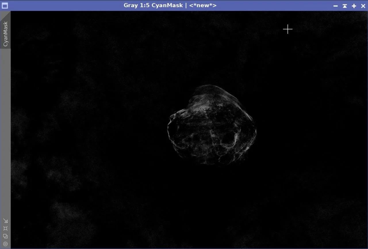
The Initial Cyan Mask
Now use HT to boost the mask image.

Boosted by HT
Now clean up the image with the DynamicPaintBrush

After Cleanup with the DynamicPaintBrush.
Use the MorpholoigcalTransform with a 7x7 pattern in Dilation to fill things in a bit. Run it up to 8 times!

Filled in a bit wit Dilation.
Now smooth the Dilation with Convolution

The Final Mask.
We can now create the Master Mask by combining the Range and Cyan Mask. Use PixelMath to do this, creating a new mask that is the union of the two input masks.
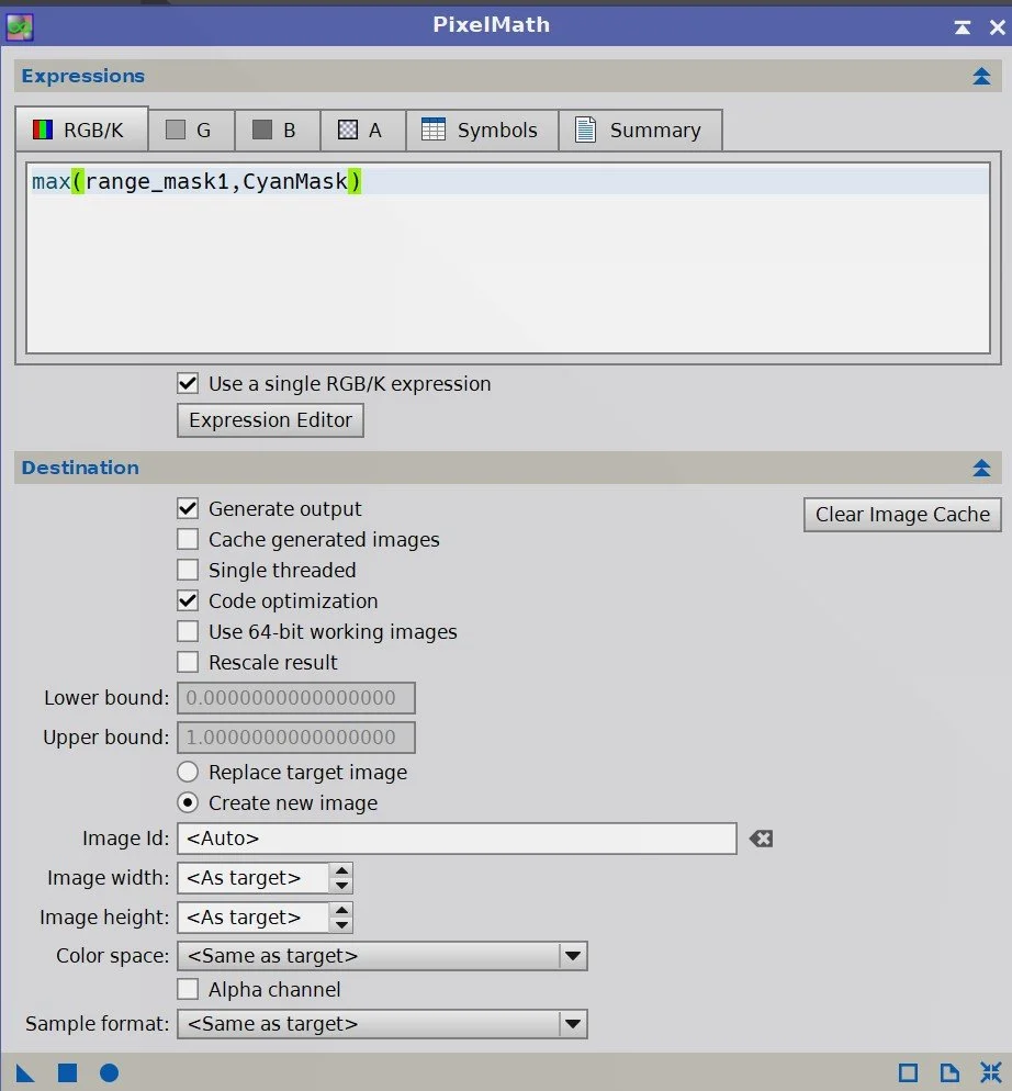
The PM equation used to create the union of the two masks.
Final Range Mask (click to enlarge)
Final Cyan Mask (click to enlarge)

The final Master mask fills in some of the O3 detail a bit better - especially the O3 “sail’ on the top!
Create the Red Mask
Create Red Mask with Bill Blanshan’s ColorMask Scripts

The initial Red Mask created with Bill Blanshan’s Color Mask Tools.
Use CT to boost the image contrast a bit

Red Mask after CT Boost.
Now blur the mask a bit using Bill Blanshan’s Color Mask Blur Script.

Now with a bit of a blur…
Next, Boost the Contrast with CT.

The final Red Mask
10. Process the HOO Image
The high end is a little blocked up. Use HDRMT with Levels = 4 to open things up a bit
Apply Master Mask
Run LocalHistogramEqualization with radius = 64, contrast level = 2.0, Amount = 0.3, 8-bit histogram
Run HDRMT with levels = 6
Apply the Red Mask
Run CT with the red curve, sat curve, and neutral curve
Apply the Cyan Mask
Apply CT Adjustment
Apply master mask
Run ColorSaturation to boost select colors - see panel shot
Run a global CT for tone scale
Apply an Inverse Master Mask and Adjust CT
Run a final HDRMT with Levels= 6 and the Master Mask
Run Nxt 0.69

After HDRMT to reduce blocked up highlights
Before LHE Applied (click to enlarge)
After LHE Applied with the Mask (click to enlarge)
After HDRMT with the Mask at Levels = 6 (click to enlarge)

Before Red Mask Adjust (click to enlarge)
After Red Mask CT Adjust (click to enlarge)
After Cyan Mask CT Adjust (click to enlarge)
ColorSat Panel Adjust. Basically boosting reds and Blues
After ColorSaturation Adjustment (click to enlarge)
After Global Tone Sale Adjust with CT (click to enlarge)
Use the Master Mask an+d CT to adjust the color of the O3 shell to be more blue and less green. (click to enlarge)
CT adjust with an Inverted Master Mask (click to enlarge)

After HDRMT with levels =5 - using the Master Mask (click to enlage)

Before and After NXT = 0.69
11. Add Stars Back In
Using PM, use a Screening equation to add the stars back in.

Here is the Screening equation used in PM to add the stars back in.
Final HOO Starless Image (click to enlarge)
RGB Stars Only

The new image with stars!
12. Export to Photoshop
Save the image as Tiff 16-bit unsigned and move to Photoshop
I tweaked things with the camera filter clarity and curves
Used the Camer Filter Color Mixer to tweak some things
I cropped things a bit tighter
Export Clear, Watermarked, and Web-sized jpegs.

First cut at the image after some Photoshop polishing.
13. Sharing and Some Second Thoughts
I was pretty satisfied wit the is final image - the O3 detail was much more apparent. Of course this was my goal, but I was really how well the convection cells in the lower part of the nebula came out.
It was true that to get these, I traded off some of the Ha color and detail.
I shared this image with others through Twitter, Facebook, and emails.
Smoke has continued shutting me down, so I have reprocessed some old data.
— 🔭Cosgrove's Cosmos💫 (@CosgrovesCosmos) July 3, 2023
I took my image of NGC6888 and reprocessed it w/ the goal of bringing out better O3 detail.
Used new methods & tools.
Old and new shown. #astrophotography pic.twitter.com/TJuKiamgJz
I received positive feedback, but the more I looked at the two images, the more I wanted to make a change. I decided to go back into Pixinsight and try to bring back some of the lost red colors of the nebula from the original image.
I did not want to lose my Photoshop changes, so I exported this image back to Pixinsight.
13. Export the Image Back to Pixinsight
Turn off watermarks
Export the image as a TIFF file
Read the TIFF File into Pixnsight.
Now I want to create a red mask that covers the nebula and the red texture within it. The problem is that because I cropped the image in Photoshop, all the masks I already have no longer fit! So I will need to craft this red mask from the start.
Create the new mask
Create a new range mask with the RangeSelection Tool
Clean up with the DynamicPaintBrush
I only want the region in the core for the red HA signal - so there is no need to expand this mask to cover the O3 regions better. This is fine where we are.
Create a new Red Mask
Use Bill Blanshan’s Color Mask Tool
Apply the new range mask and invert.
This protects the core area we want to change and exposes the area we wish to clear.
Use PM with Equation “0” to wipe out the unprotected part of the mask
Remove the mask
Use CT to boost this mask
Apply the new red mask to the image and use CT to boost the color of the reds.
The resulting image looks less muddy and dark to me.
Initial Range Mask (click to enlarge)
Initial Red Mask (click to enlarge)

New Range Mask After cleanup with the Dynamic PaintBrush - outside used a black brush, inside used a white brush. (click to enlarge)
Now we apply the range mask to the red mask and invert it. (click to enlarge)
Red Mask After PM Applied to remove outer area. (click to enlarge)
Final Red Mask after CT Boost. (click to enlarge)
Starting Image From PhotoShop (click to enlarge)
After Applying the Red Mask and using CT to boost the red very slightly. (click to enlarge)
I created a video showing this last editing sequence for my 2-Minute Tutorial Series. That video can be seen below:
14. Export Back to Photoshop and finish the Image
Save the image as Tiff 16-bit unsigned and move to Photoshop
Export Clear, Watermarked, and Web-sized jpegs.
The fInal Image!
Adding the next generation ZWO ASI2600MM-Pro camera and ZWO EFW 7x36 II EFW to the platform…