
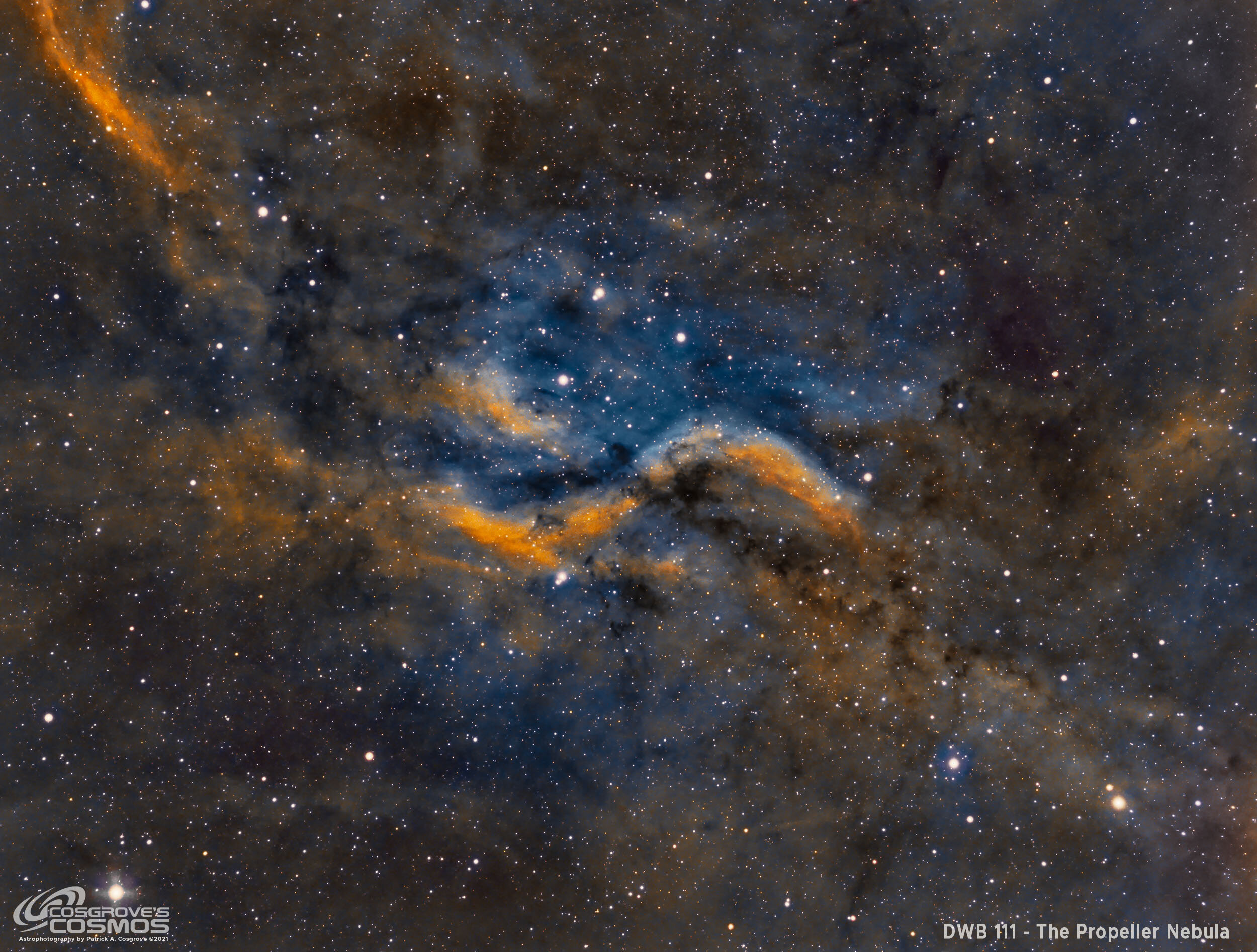
DWB 111/119 - A Reprocess of The Propeller Nebula - in SHO ~ 10 hours
Date: Aug 7, 2023
Cosgrove’s Cosmos Catalog ➤#0126

My second take on the DWB 111/119 data - taken with a mono camera and rendered using the Hubble Palette (click image for full resolution va Astrobin.com)
Table of Contents Show (Click on lines to navigate)
Introduction
Here we are in early August of 2023, and my year has been abysmal so far regarding my astrophotography. I have only had two nights of data capture thus far - and those two nights have some smoke issues!
So I have been going back and doing some reprocessing projects. I have been selecting targets where I had collected a reasonable amount of data - and had an initial image that I was never delighted with.
Could new tools and techniques acquired since the data was captured make a difference? In some cases - it can make a huge difference. Would it make an improvement here?
I always thought that my original image looked like it some kind of pastel drawing. I just did not like it. The original Project post can be seen HERE. The original image can be seen here:
My original Image.
I will talk about this more in-depth - but I had a hard time getting this image to a point where I was happy with it.
Some images practically process themselves. Others are challenging, but I find a way to proceed and get a result I like immediately. Some seem to vex me.
They seem hard to process. The results are not pleasing. It can seem challenging to figure out what look is the right look.
This one vexed me. I’m OK with the final result - but unsure how much I really helped it.
You will have to be the ultimate judge!
About the Target (copied from the original post)
The Propeller Nebula is part of a vast and rich region in Cygnus known as Cygnus X Complex. The Propeller is often designated as DWB 111; however, this is incorrect, as we will see. The proper designation is Simeiz 57.
DWB and Simiez designations are not so commonly known, so first, a little history.
The Simeiz Catalog was created in the 1950s by the Crimean Astrophysical Observatory in Simeiz, Ukraine. This catalog is focused on HII regions and documented 306 of them. The Propeller Nebula is item 57 in this catalog.
The DWB catalog was created in the 1960s by H. R. Dickel, H. Wendker, and J. H. Bieritz, and it cataloged the HII regions they were studying in the Cygnus X Complex. While DWB 111 is often used as the designation for the Propeller, it only deals with the southern arm of the Propeller, while DWB 119 deals with the northern arm.
So you can call it DWB 111/119 or Semeis 57. I will follow the standard convention and call it DWB 111 in this posting.
HERE is the best link I found dealing with the designation for the Propeller. It also shows all designations and how they relate to one another.
While we don't really know how far the Propeller is from the Earth, the Cygnus X Complex, in general, has been determined to be about 4,600 light-years away.
This object is primarily known by Astrophotographers. It is a faint object that shines with a feeble red light - which your eyes are not all that sensitive to. You will need a larger aperture telescope - perhaps 14” or larger in diameter - and probably use a filter to enhance contrast to see it visually.
Astrophotographers have the advantage of storing light over time and integrating it - making such faint and tenuous objects visible. Even so, I needed 12 hours of integration under good conditions to get this image!
The Annotated Image

Annotated image of DWB 111/119 - Note that there is not much annotation! This object was too faint to make into the traditional catalogs used for such annotation! (this image was created using the Pixinsight ImageSolver and AnnotateImage scripts)
The Location in the Sky

This finder chart was created using the Pixinsight ImageSolver and FinderChart scripts)
About the Project
Since the data was captured for the original project, I will let that posting provide the details around the selection, set up and collection of the data. It also covers some of the data analysis as well.
However, I did do another pass on the data - and decisions that I made this time around may be different than on the first pass. The blink information is provided in the Image Processing Walkthrough below.
Image Processing
Whats Different This Time Around?
This time around, there are several things that will be different. These are listed below:
The use of BlurXTerminator instead of traditional Deconvolution
The use of NoiseXTerminator instead of ACDNR
The use of a starless workflow - leveraging StarXTerminator
The use of Bill Blanshan’s NBNormailization4.1 Script to adjust the initial SHO color image
The use of Bill Blanshan’s ScreenStars to add stars back in
Note that I also am NOT using a Lum vs Color workflow for this image. I am starting to shy away from that approach for narrowband images - though I used it for many projects in the past.
The split Lum/Color approach made a lot of sense when I was using traditional Deconvolution:
I could apply it to the Lum image alone and save a lot of work
I avoided having different sized stars from applying Deconvolution the each color image before they are combined.
But now I am using BlurXTerminator. BXT does best when dealing with a full color image. This avoids issues I have seen in the past - so there is now less need to use the Lum/Color approach.
There was another problem that I was seeing with this approach.
Since Ha, O3, and S2 images can look SO very different from one another - creating the synthetic Lum image can obscure some details from images with lower signal levels. This is most often the O3 or S2 channels. Now I tend to want to enhance each of those as much as possible to bring out their detail and avoid smooshing them together with the LRGBCombination Tool.
Challenges I Ran Into This Time
As I mentioned before - this time around I had a lot of trouble working on this image.
I thought that I had overdone it the first time and I wanted to back off and create something that looked more natural this time.
So I processed the image to a point where it had a much less “processed” look and created the comparison below:
The original Image (click to enlarge)
My first reprocess attempt (click to enlarge)
I shared this new image with friends and on Facebook and Twitter.
I was actually kind of surprised when I received a very mixed response!
Most people though I went too far in reducing the stars. Most thought the image was darker and less colorful. Finally - many thought I had reduced the dust detail too much.
I was not expecting this kind of response - but then again - this is why I tend to share early versions of an image for feedback. Sometimes you can get too invested in one approach that is not an optimal one. The feedback forces you to reassess - and that is a good thing.
I thought I had done a pretty good job on not going overboard on the processing (which I sometimes have the tendency to do!). As I reconsidered - the image I can see some merit to the feedback.
I decided to create another version that would address these concerns. The image I created can be seen on the left below.
It brings up the contrast and the color, backs off on the star reduction, greatly enhances the dust detail. Being a high-color kind of guy - thought I was done with the image. I am not sure how much better it is compared to the initial image - but it certainly is different.
I thought I was all set and even started creating this post using that version of the image. But one day I opened up my laptop and loaded my page - and my instant reaction was that I had gone too far! It had TOO MUCH color!
So I went back and dialed down the color and the contrast a bit - and I think this works better.
But - you tell me - which o you like better?
The higher color version (click to enlarge)
The slightly lower color Final Version (click to enlarge)
The new image is a bit less garish - and now I think I am finally done!
More Information
Cloudy Nights: A nice write-up about DWB 111/119 for a visual challenge
Wikipedia Entry: The Cygnis X Complex
Distant Lights: Overview of the Propeller Region
Astronomy & Astrophysics: The Science article for the study of HII regions in Cygnus X COmples that includes the DWB Catalog.
Capture Details
Light Frames
Taken on the night of September 1st, 6th, and 8th, 2021
Ha Filter: 50 x 300 seconds, bin 1x1 @ -15C, gain at unity
OIII Filter: 48 x 300 seconds, bin 1x1 @ -15C, gain at unity
SII Filter: 45 x 300 seconds, bin 1x1 @ -15C, gain at unity
Total of 11.9 hours, After culling for this reprocessing project, this was reduced to 10 hours and 5 minutes.
Cal Frames
Darks: 30 x 300 seconds, bin 1x1 @ -15C, at unity
Flats: 12 Ha, OIII, & SII for each night,
Flat-Darks: 30 for each night
each night’s lights calibrated with that night’s flats and Flat Darks
Capture Hardware
Click below to visit post about the Telescope version used for this image
Scope: William Optics 132mm f/7 FLT
APO Refractor
Focus Motor: Pegasus Astro Focus Cube 2
Cam Rotator: Pegasus Astro Falcon
Guide Scope: Sharpstar 61EDPHII
Guide Focus Motor: ZWO EAF
Mount: Ioptron CEM 60
Tripod: Ioptron Tri-Pier
Camera: ZWO ASI1600MM-Pro
Filter Wheel: ZWO EFW 1.2 5 x8
Filters: ZWO Gen II 1.25” LRGB,
Astronomiks 6nm 1.25” NB
Guide Camera: ZWO ASI290MM-Mini
Dew Strips: Dew-Not Heater strips for Main and Guide Scopes
Power Dist: Pegasus Astro Pocket Powerbox
USB Dist: Startech 8 slot USB 3.0 Hub
Polar Align Cam: Polemaster
Image Processing Walkthrough
(All Processing is done in Pixinsight - with some final touches done in Photoshop)
1. Blink all Data
Note: These images have already had some images removed in the initial processing. Here I removed even more.
HA:
looks good - some trails
2 rejects - clouds
10 rejects - focus
O3 :
Little to no nebula showing in subs
Clouds impacting a subset of frames - 11 removed
S2:
looks good - none remove.
Something seems to be going wrong in autofocus on the platform - most of these I caught and forced autofocus to run during the session.
Flats - all look good.
2. Run WPBB 2.5
Load al lights
Set exp tolerance to 0
Load flats
Load darks
Set exp tolerance to 0
Set max quality
Set keyword NIGHT
Output folder - wbpp2
Everything is set to run except linear fix
Integration - large-scale pixel rejection set for high and low at 2x2
Map missing darks and flats
The pedestal set to auto
CC to applied to all
Set to auto crop
Ran without error.

Post Calibration View of WBPP


Pipeline view
2. Load Master Images and Rename

The Master Ha, O3, and S2 images.
3. Run DBE for each image
No gradients seen, so DBE was NOT run.
4. Create the Initial SHO image
I want to create the SHO color image right away so I can run BXT on it in linear space
Run ChannelCombination for the SHO mapping.
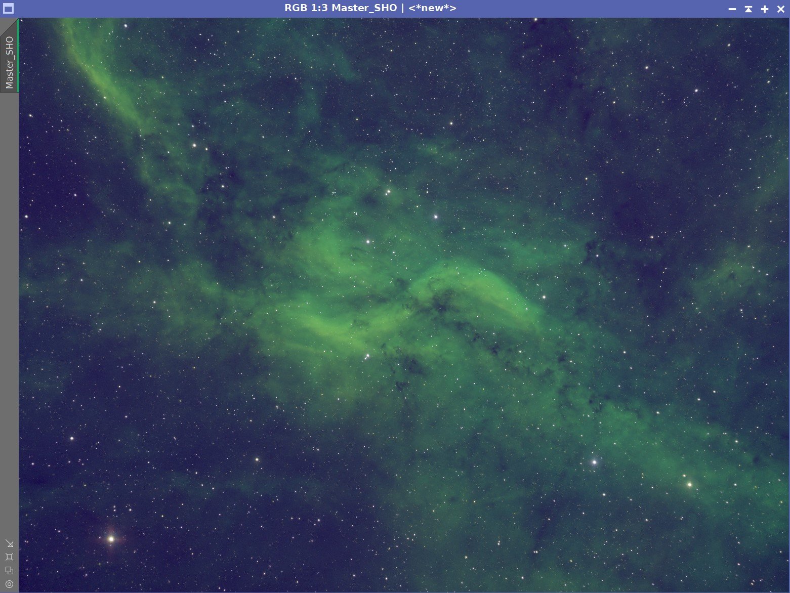
The initial SHO image
5. Process the Linear Image
Do Deconvolution:
Run PFSImage on the color SHO image. This will measure the FWHM stars sizes in X and Y.
The resulting star sizes measured are X=2.59 and Y=2.3
We will use this with BXT in the Non-stellar Adjustment area. We will use a size of 2.50
Experiment with BlurXTerminator Settings for stellar adjustments - see panel snap shot for final version used
Run BlurXTerminator
Run NoiseXTerminator 0.5. This light application of NXT will just “knock the fuzz off” the linear image.

PFSImage Analysis Results

BXT settings used.
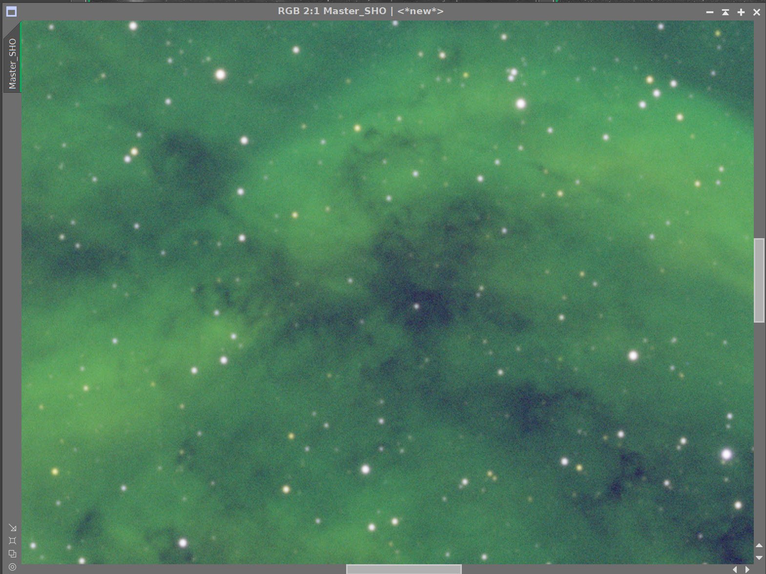
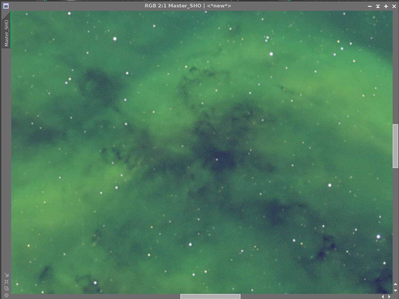
Master SHO Before BXT, After BXT and NXT = 0.5
6. Go Starless
Run StarXTerminator with “Generate Star Images”, and “Unscreen Stars” selected - see screen snap below.
This will create a starless and an stars-only image using a screening equation.
Run the NBNormailize4.1 script by Bill Blanshan using default values.
I don’t normally use this script, so it is a bit of an experiment this time around.
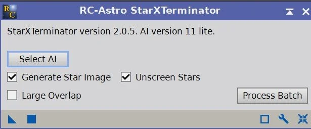
SXT Parameters run
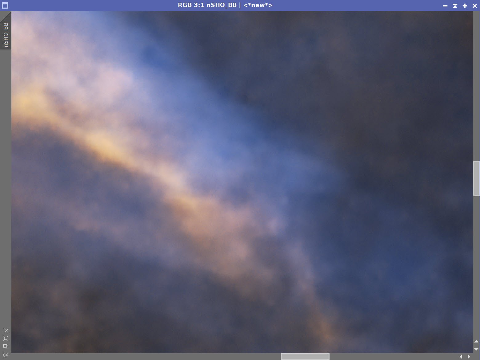
The Master SHO image before running StarXTerminator
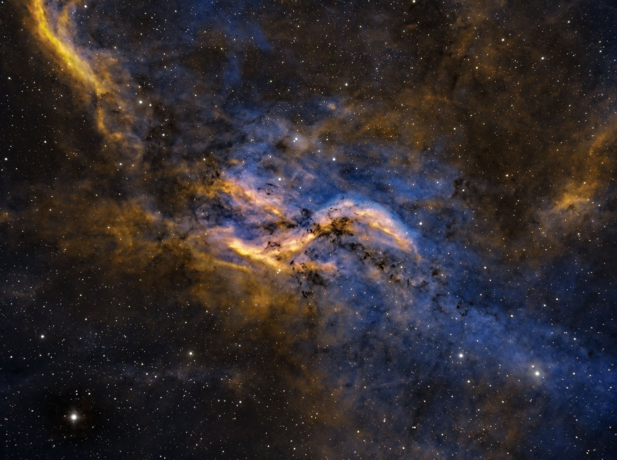
The resulting Starless Image (click to enlarge)
The resulting Stars image (click to enlarge)

The normalized Master SHO Starless image - ready to go nonlinear!
7. Go Nonlinear
Use the STF->HT method to go nonlinear
Adjust the image with a simple CT
The initial Nonlinear Image (click to enlarge)

After the initial CT adjust (click to enlarge)
8. Create the Initial Color Masks
I typically use a lot of masks in my processing and I usually start with a series of color masks as seen below. Typically I blur them out a bit, but no for today for reasons and I actually kind of unsure of myself! It just felt right to me.
Using the Bill Blanshan Color Mask Scripts to do the following
Create a Yellow Mask
Apply CT to the Color Mask to enhance the mask
Create a Red Mask
Apply CT to the Color Mask to enhance the mask
Create a Blue Mask
Apply CT to the Color Mask to enhance the mask
Create a Green Mask
Apply CT to the Color Mask to enhance the mask
The initial Yellow Mask (click to enlarge)
Yellow Mask after CT enhance (click to enlarge)
Initial Red Mask (click to enlarge)
Initial Blue Mask (click to enlarge)
Initial Green Mask (click to enlarge)
Red mask after CT adjust (click to enlarge)
Blue Mask after CT Adjust (click to enlarge)
Green Mask after CT Adjust (click to enlarge)
9. Complete the initial Process of the SHO Image
Here, all I am really doing is applying the various color masks and playing with the CurvesTransformation tool (CT) adjusting the neutral curve and saturation to get a look I like.
Apply yellow mask
Adjust with CT
Apply red mask
Adjust with CT
Apply blue mask
Adjust with CT
Do a global CT adjust
Run LocalHisorgramEqualization (LHE ) with the Green Mask using a radius of 64, contrast limit of 2.0, an amount of 0.75, and an 8-bi histogram. This will enhance the detail of the yellow/orange portions of the nebula.
Apply another round CT adjusts with the Green and Yellow Mask
Run NXT with a value of 0.65
CT Adjust with Yellow Mask (click to enlarge)
CT Adjust with Blue Mask (click to enlarge)

After LHE adjustment using the Green Filter (click to enlarge)
CT Adjust with Red Mask (click to enlarge)
Global CT Adjust (click to enlarge)
CT Adjust with Green Mask (click to enlarge)

Before and After NXT = 0.65
10. Take the Stars Only Image Nonlinear
The star are already pretty small from DBX, so no need to adjust STF to shrink them - I am just tweaking things until Iam happy with the look.
Adjust Master Stars image with STF
Use STF->HT to go nonlinear

The nonlinear Stars Image
11. Combine Images and Share for Feedback
Use Bill Blanhan’s ScreenStars Script to add star images back in. I used to use a screening equation in PixelMath to do this, but I find this a lot more convenient!
Share this initial Image with friends and on Twitter and Facebook
Feedback was:
Stars too reduced
Colors too muted image is dark
Dust regions not brought out
Let’s take another pass and see if we can address these issues

The ScreenStars Script panel

This is the image shared for early feedback
12. Revisiting the Color SHO Image
Apply Global CT
Apply Global CT with the Green Mask
Create a Range Mask - edit it to that just the propeller is targeted.
Create a GAME Mask covering upper left feature that looks a little blown out
Apply CT with RangeMask
Apply CT with GAME Mask
Apply HDRMT with the RangeMask in place. This area is bright and a little blocked up. I use HDRMT to pull contrast and detail back in.
Apply CT with the RangeMask in place - this will restore some of the contrast lost in the HDRMT operation.
Create a Dark Mask using the DarkStructureEnhance script and the extract mask feature
Apply the Dark Mask
Do a CT
Do a LHE operation 40,2,0.6,8-bit
These two operations will enhance the dust features
Starting Point (click to enlarge)

After CT with the Green Mask Applied (click to enlarge)
After Global CT (click to enlarge)
Initial Range Mask (click to enlarge)
The Range Mask after clean up with the DynamicPaintBrush (click to enlarge)
The GAME Mask (click to enlarge)
After CT with RangeMask (click to enlarge)
After HDRMT with Level 7 using the RangeMask (click to enlarge)
After CT with GAME Mask (click to enlarge)
Initial DarkMask from the DarkStructuresEnhance Script (click to enlarge)
After CT Adjust with DarkMask (click to enlarge)
DarkMask after CT Adjust (click to enlarge)
After LHE apploed using the DarkMask (click to enlarge)
13. The Final Process of the Stars
The brighter star has microlensing artifacts from the sensor. This is common with the ASI1600MM-Pro camera. So to fix that, we will create a red mask. This will target the color artifacts.
Apply the mask and then reduce the saturation of the red regions.
Now remove the mask and adjust the star images with CT to reduce other weird colors and do a final adjust ton the stars
The Starting Star Image
The Red Mask create to cover bright star artifacts
Zoomed in view of the brightest star (click to enlarge)

After CT adjust with the Red Mask (click to enlarge)
After CT to drop over all color
The Final Star Image
14. Add Stars Back in
Use ScreenStars Script t add the stars back in
The Final Starless Image (click to enlarge)
The final Star Image (click to enlarge)

Final Image - ready for Photoshop Polishing
14. Export To Photoshop for Polishing
Adjust global Clarify and Curves
Use ColorMixer to Adjust Blue and Orange darkness and color sat
Do some lasso work to adjust some faint local features
Add watermarks
Create a high and mid-color version
Export

The Higher Color Version - Probably too high!
Slightly lower color version - and what I choose as my final version!
I was very excited to get the ZWO ASI2600MM-Pro camera a while back. I ordered it when it was announced and then prepared to wait a long time to get it. When I did get it - I decided to put it onto the AP130 platform. That meant that I could move the ZWO ASI1600MM-Pro, along with its filter wheel over to my William Optics Platform. This now means that all of the platforms have been moved over to a mono camera and my ZWOASI924MC-Pro is now not in use.