
Markarian’s Chain - A Famous Galaxy Cluster with 4.6 hours LRGB
Date: May 25, 2025
Cosgrove’s Cosmos Catalog ➤#0137

The first image from my Whispering Skies Observatory from my little FRA400 Astrograph! (click on the image for a high res view via Astrobin.com)
Table of Contents Show (Click on lines to navigate)
Published in the November 2025 Issue of BBC Sky At Night Magazine!

About the Target
A Galactic Conspiracy in Virgo
Sometimes, the universe lines things up just right—and Markarian’s Chain is a perfect example. This striking string of galaxies in the constellation Virgo isn’t just an optical illusion. Many of its members are actually moving together through space like a galactic conga line—minus the music and plus a few billion stars each.

Benjimin Markarian (1913-1985) as seen on an Armenian Stamp.
Named after Armenian astrophysicist Benjamin Markarian, who in the 1960s observed that several galaxies in the Virgo Cluster shared a common motion, the Chain is part of the larger Virgo Cluster, located roughly 50 to 60 million light-years away. That’s close enough to resolve its features with modest amateur equipment, but far enough to keep things tidy in our cosmic neighborhood.
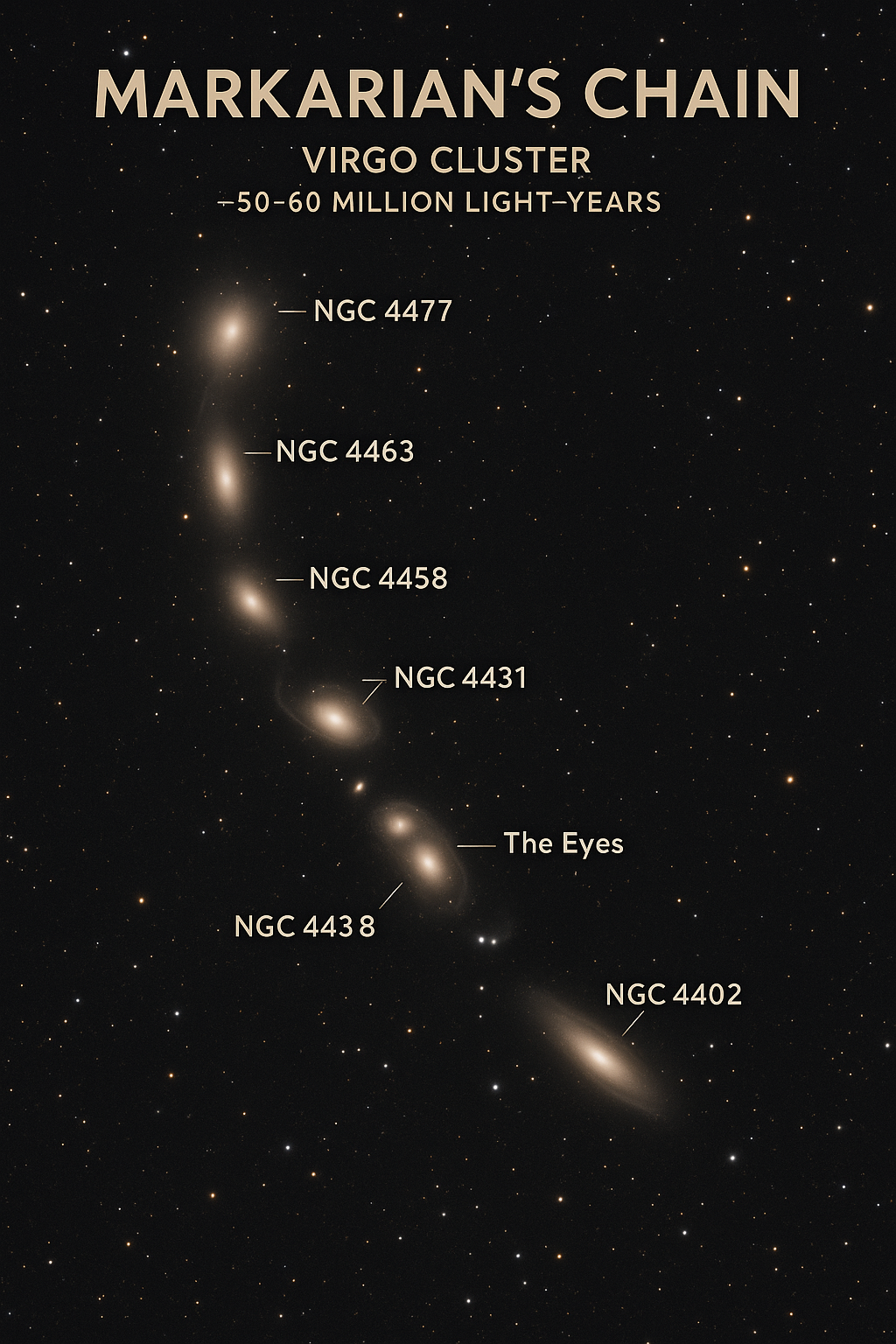
The main arc of the Chain spans about 1.5 degrees of sky and includes a photogenic mix of elliptical, lenticular, and spiral galaxies. Here’s a breakdown of the headliners:
NGC 4477 – Barred lenticular galaxy (SB0)
NGC 4473 – Elliptical galaxy (E5)
NGC 4461 – Lenticular galaxy (SB0)
NGC 4458 – Elliptical galaxy (E0-1)
NGC 4438 – Disturbed spiral/peculiar galaxy (Sbp pec), tidally warped - Larger companion in the “Eyes”
NGC 4435 – Lenticular galaxy (SB0); the smaller companion in “The Eyes” pair
NGC 4402 – Edge-on spiral galaxy (Sb) with visible dust lanes, just off the arc
Messier 84 - A giant elliptical or lenticular galaxy(E1)
Messier 86 - A giant elliptical or lenticular galaxy(E3)
These galaxies aren’t just pretty—they’re also busy. For example, NGC 4438 and NGC 4435 (together known as “The Eyes”) show signs of a past close encounter, with visible distortions and tidal debris. It’s like watching a cosmic traffic accident in slow motion—if the vehicles were 100 billion solar masses and the crash lasted 100 million years.
Why It Matters
Markarian’s Chain isn’t just photogenic—it’s a window into the processes of galaxy clustering, interaction, and evolution. It provides astronomers with a real-world lab to study how galaxies behave in dense environments, how gravity molds their structures, and how galactic drama unfolds on cosmic timescales.
Ideal Observing Window
The Chain is best viewed during spring months (March–May) in the Northern Hemisphere. With a wide-field setup, you can capture multiple galaxies in a single frame, plus a slew of background galaxies sprinkled throughout the field like celestial confetti.
The Annotated Image

Created in Pixinsight using the ImageSolver and AnnotateImage scripts.
The Location in the Sky

This annotated image created with Imagesolver and FInderChart Scripts in Pixinsight.
About the Project
This is the first imaging project from my Askar FRA400 platform, taken from my new observatory!
Picking the Target
I was in scramble mode.
The first clear night without the Moon was coming up just after I got the scope installed in my new Whispering Skies Observatory. I was still trying to ensure that the new Mele Micro-PCs were set up correctly and that I had configured NINA on all four telescopes correctly. This was pretty much absorbing all of my time.
I was also having a problem with the NINA Autofocus routine with my FRA400. Autofocus curves looked great on the left side of the screen but were flat on the right side. This usually involves a problem with backlash on the focus gearing. While I improved it, I never really got it where I wanted it. I got it well enough that it would do a successful Filter Offset series, and I would have to go with that.
However, the main point is that I did not have the time I normally have to do my planning process prior to a shoot.
I cheated and used ChatGPT to offer a range of possible targets for this scope.
One of those was Markarian’s Chain.
I was familiar with this and knew that it spanned a pretty good chunk of sky—about 1.5 degrees. This is just the kind of target that my FRA400 is designed to pursue—those bigger targets.
Now I should mention - in all honesty - I am not that thrilled with Galaxy Clusters.
Well, let me frame that better.
I love the concept and idea behind a Galaxy Cluster!
I mean, come on, the idea of a group of galaxies 50 million light-years away traveling together in space, gravitationally bound, and interacting just blows the mind and ignites the imagination. Right?
But from an imaging perspective, they can be dull. Tiny, itty-bitty fuzzy specks of galaxies with little to no color or detail? YAWN…..
These galaxies are sitting on a pretty sparse field of stars. After all, to see them, we tend to look away from the Milky Way and its rich star fields, out into open space. YAWN…
But this time around, I decided to go for some Galaxy Clusters - just to say I did - maybe have some new imaging experiences - maybe I would like them after all!
Markarian’s Chain is well known - so why not?
I went into NINA and began to frame my shot. I centered on M86 to get started. I saw what I thought would have been the main portion of the Chain, but I also saw a lot more glaxes in the area. So I framed things to maximize the number of galaxies I could fit into the frame.
Data Collection
We had clear nights on April 22nd and again on the 27th. I shot both nights—all night.
Everything seemed to be going well. Tracking looked good. I figured that I probably had 8 hours of integration—not bad for an f/5.5 scope on this kind of target.
On April 24th, I shot a completely new calibration series so I would be ready to process when I completed data collection.
The weather changed, and we were expecting weeks of cloudy nights, so I figured it was time to start processing.
I first processed the M106 Image I shot on the SCA260, as I was eager to see how that came out. You can read all about that project HERE.
Then I decided to work on this project next.
The first thing I always do is blink the data.
I did that here and was a bit surprised by what I saw. I thought we had two good, clear nights. But when I looked at my frames, I saw a lot of Subs that were impacted by thin clouds coming through!
Blink of Lum subframes.
You will see the details below in the complete processing walkthrough, but the culls resulting from the blink analysis and removing subs with SubFrame Selector ended with only 4.6 hours of total data remaining!
I think this is the biggest frame loss I have encountered since I began my astrophotographic journey!
With that, I began my preprocessing with Pixinsight’s WBPP.
Processing Overview
Since the galaxies in the Chain were small, I decided to do a 2X drizzle process on the images in WBPP to maximize the resolution I was dealing with.
Then my plan was to do a LRGB Starless workflow.
The high-level flow of this approach can be seen below.
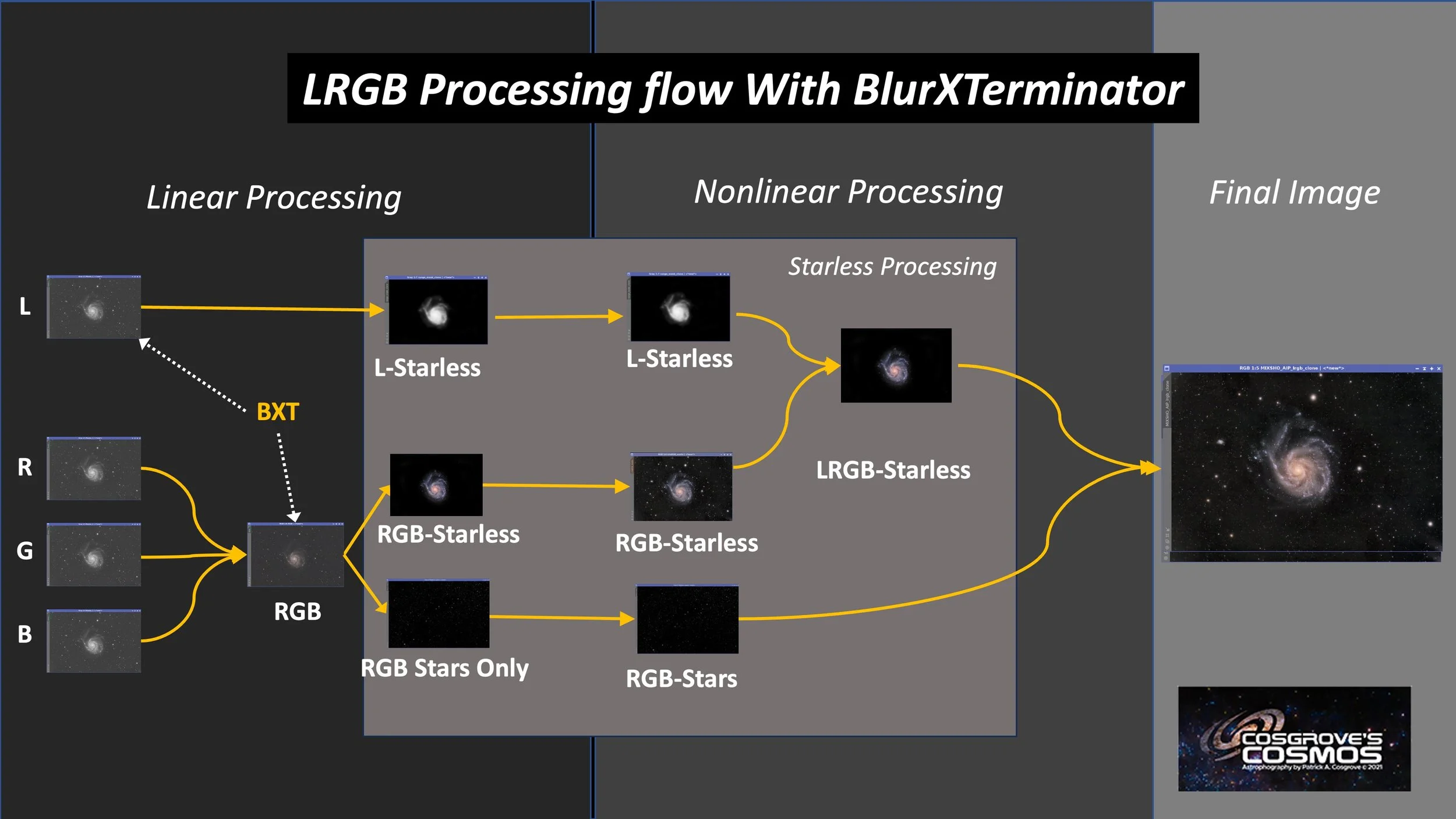
My typical LRGB Starless Workflow.
These days, I tend to create my Master RGB linear images right away. Then I do a pretty standard series consisting of DBE, BXT- Correct-only, SPCC, Full BXT, and a light NXT on the color image itself. I used to do this on each sub-image (R, G, &B). But this saves time and seems to give a better result
Then I do the DBE, BXT-Correct-Only, BXT-Full, and NXT sequence on the luminance master next.
At this point, I use STX to go starless and then jump to nonlinear.
I enhance the Lum for detail and sharpness.
I enhance the RGB for color and low noise. Then these two images are folded together.
I process the RGB stars, and fold those in, and I am done.
I must admit that I really worked at this.
The galaxies were very small, and I was trying to bring out what color and detail I could. Given that my integration was distressingly short, there was only so much I could do.
The final image was - in my opinion - lackluster. I was just not impressed with the result.
Here is what I was looking at:

My initial Image. I was just not liking the composition. Yeah - there are a lot of galaxies captured - but the image was kind of Blah.
I composed this image to maximize the galaxies captured. I achieved that goal, but I was just not happy with the resulting image.
So, as I often do, I shared it with my local circle of Astro Imaging Friends.
One of them (Thanks, Dave!) made an interesting suggestion. “Why not rotate the image 90 degrees CCW and center it on the chain itself?”
I thought this was an interesting idea. I did just that and created the following test images, which I again shared.
The first image had the same aspect ratio of the original image and I arranged the image as a smile.
With the second image, I flipped the smile upside down and used a 16 x 9 aspect ratio.
Sam aspect ratio as the original image - the chain positioned as a ‘smile.’

This one has a 16 × 9 aspect ration and the ‘smile’ is now a frown!
After more feedback and considering what I liked, I decided to go with the orientation of the second image, but the aspect ratio of the first! This is what you see in the final image.
Look below for the complete step-by-step processing walkthrough! Note: This walkthrough is based on Pixinsight.
Final Results
I have to say I was a little disappointed with this image.
It was short on integration time. The detail and color were not spectacular by any means. Part of this is the subject matter. It’s just not as impressive as other types of targets can be.
The galaxies in the chain only measure about 2-3 arcminutes in size, so what would you expect?
On the other hand:
It is one of the first images from my new observatory, so that is pretty cool!
The rotation and crop made for a much more interesting composition, better than what I started with.
The galaxies, small as they are, do show some color and detail, which you often don’t see in images of the Chain.
The idea that this group is 50 million light-years away, traveling through the universe together, and in some cases, gravitationally interacting - IS very cool!
More Information
🔭 General Background & Observing Guides
Wikipedia – Markarian’s Chain
A comprehensive overview of the chain’s discovery, structure, and key galaxies.
BBC Sky at Night – Complete Guide
Offers observing tips, equipment recommendations, and a finder chart for the chain.
🔗 https://www.skyatnightmagazine.com/astrophotography/galaxies/markarians-chain
Astronomy.com – Explore Markarian’s Chain
Provides a historical perspective and guidance for amateur astronomers.
🔗 https://www.astronomy.com/science/explore-markarians-chain
🧬 Scientific Insights & Interesting Facts
James Webb Discovery – 100 Fascinating Facts
Delves into the chain’s role in understanding galaxy formation, dark matter, and cosmic evolution.
🔗 https://www.jameswebbdiscovery.com/universe/100-fascinating-facts-about-markarians-chain
EarthSky – Today’s Image Feature
Highlights the chain’s significance within the Virgo Cluster and its gravitational interactions.
🔗 https://earthsky.org/todays-image/markarians-chain-of-galaxies/
🌌 Hubble & Webb Telescope Imagery
NASA APOD – Markarian’s Chain of Galaxies
A high-resolution image capturing the chain’s structure and key galaxies.
NASA APOD – The Eyes in Markarian’s Chain
Focuses on the interacting galaxies NGC 4438 and NGC 4435, known as “The Eyes.”
📚 Historical Context & Discovery
Messier Objects – Markarian’s Chain
Details the discovery of individual galaxies within the chain and their cataloging history.
Astronomy Now – The Eyes Have It!
Discusses the significance of the interacting galaxies within the chain and their observational history.
🔗 https://astronomynow.com/2022/04/19/markarians-chain-the-eyes-have-it/
Capture Details
Lights Frames
Taken the nights of April 22nd and 27th, 2025
32 x 120 seconds, bin 1x1 @ -15C, Gain 139.0, ZWO Lum Filter - 1.25 inch
32 x 120 seconds, bin 1x1 @ -15C, Gain 139.0, ZWO Red Filter - 1.25 inch
34 x 120 seconds, bin 1x1 @ -15C, Gain 139.0, ZWO Green Filter - 1.25 inch
41 x 120 seconds, bin 1x1 @ -15C, Gain 139.0, ZWO Blue Filter - 1.25 inch
Total - after culling bad subs - of 4 hours and 38 minutes.
Cal Frames
25 Darks at 200 seconds, bin 1x1, -15C, gain 139
30 Dark Flats at Flat exposure times, bin 1x1, -15C, gain 139
One set of Flats done:
15 Lum Flats
15 R Flats
15 G Flats
15 B Flats
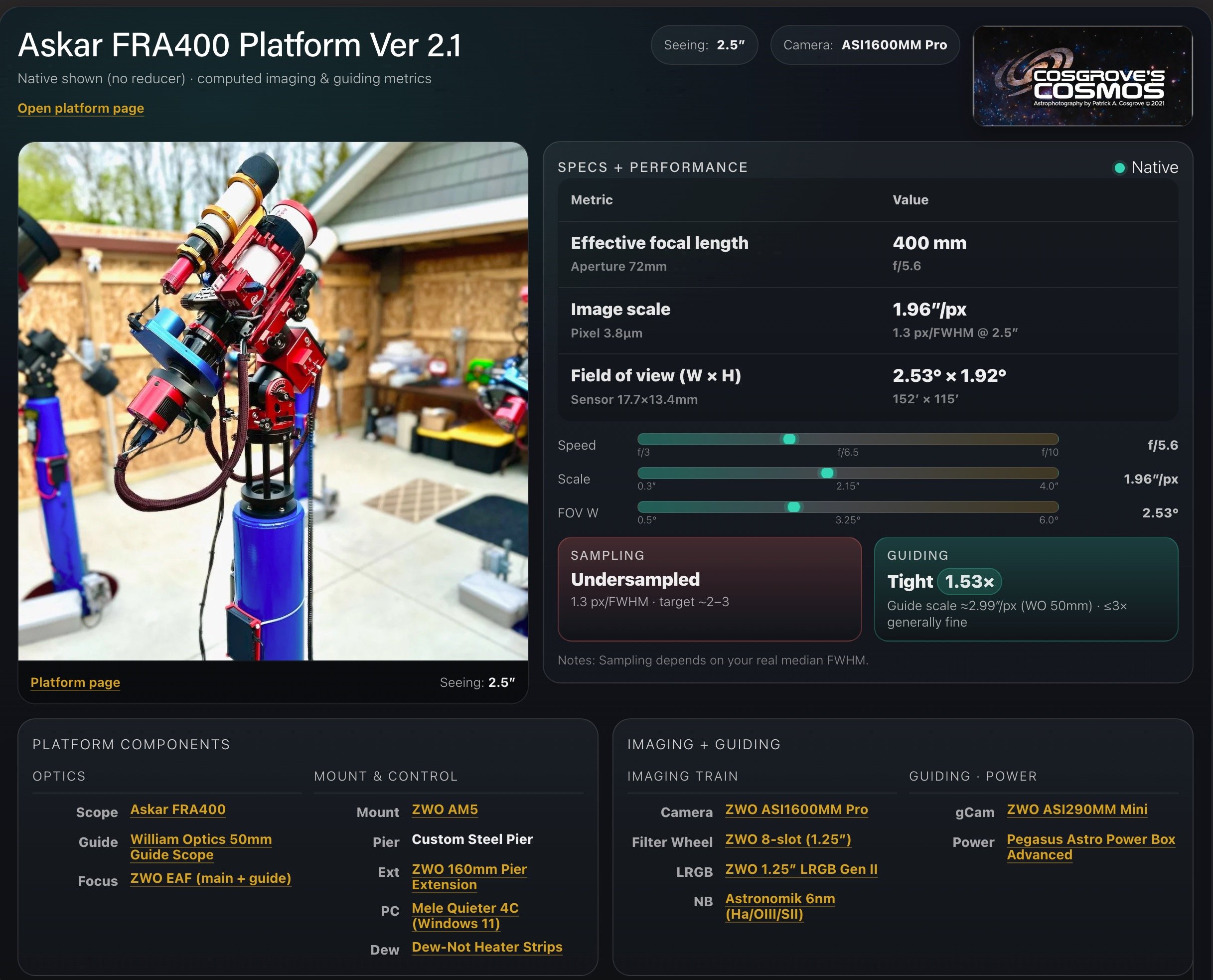
Platform used for this project
Software
Capture Software: PHD2 Guider, NINA
Image Processing: Pixinsight, Photoshop - assisted by Coffee, extensive processing indecision and second-guessing, editor regret and much swearing…..
Image Processing Walkthrough
(All Processing is done in Pixinsight - with some final touches done in Photoshop)
1. Blink and SubFrameSelector Analysis
Blink:
Lum Subs:
Some thin clouds are coming through on a surprising number of subs!
15 frame removed!
Red Subs:
A few satellite trails were noted
Thin clouds on some
11 removed!
Green Subs:
A few satellite trails were noted
9 removed!
Blue Subs:
A few satellite trails were noted
7 removed
All Flats and Darks:
All looked good!
However, I noticed that my Darks were for 200 seconds rather than 120 seconds. I will have to optimize them in WBPP.
SubFrameSelector
Lum

Lum SFS report.
As you can see, there are 5 frames remaining that have enlarged stars. I removed those as well. I have one that had larger eccentricity, but I am counting on the WBPP rejection logic to handle that.
Red

Red SFS Report.
Red had eight more frames removed. The first night seemed problematic. Again, there was only one really eccentricity problem, which I left.
Green

Green SFS report.
8 more frames removed - a very similar pattern to the red.
Blue

Blue SFS Report
Blue was the best of the bunch for some reason. Only 2 more frames were removed.
Summary
A total of 65 subs were removed due to clouds! That’s a total of 1.8 hours of integration lost. I think this is the worst case I have had. Now we have to make the best of the data we have!
2. WBPP 2.8.6
Reset everything
Load all lights
Load all flats
Load all darks (note: darks for 200 seconds, not 120 as they should have been!)
I choose to optimize darks.
Select - maximum quality
Reference Image - auto - the default
Select the output directory to wbpp folder
Enable CC for all light frames
Pedestal value - auto
Darks -set exposure tolerance to 0
Lights - set exposure tolerance to 0
Lights - all set except for linear defect
set for Autocrop
Set for 2X Drizzle
Executed in 39 minutes - no error!

WBPP Calibration View
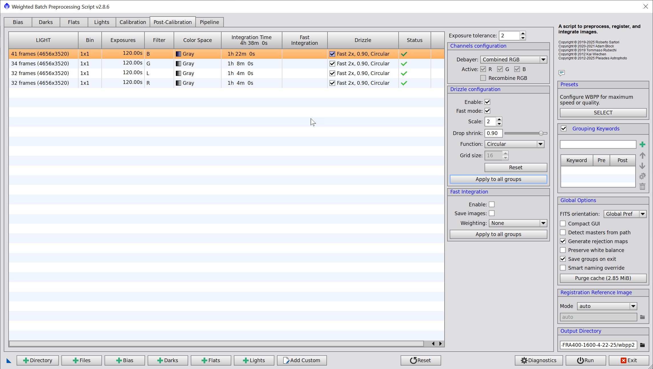
WBPP Post Calibration View

WBPP Pipeline View
3. Load Master Images
Load all master images and rename them.

Master L, R, G, & B images
4. Process Linear RGB data
The gradients were mild, but with so little nebulosity, there was no trouble running DBE:
Set up the sample pattern as shown
Fix with subtraction
Run BXT correct-only. Best to fix any star issues before SPCC
SPCC and calibrate the color. Use the Ideal QE curve and ZWO RGB filters. See the panel setup below.
Run PFSIMage to get an idea of the star sizes. X = 3.52 Y = 3.39
After experimenting with BXT settings, I used 5.59 for non-stellar restoration, which was much larger than the PFSImage results.
Run BXT Full correction - see settings used on the panel shot below.
Apply NXT to remove noise. Be aggressive here, as I want smooth star edges. Used model 3 and settings shown in panel snapshot below.
Use STX with Saving Stars and Unscreen Stars selected to create RGB Stars and RGB Starless images. Set to large sample box size

The initial RGB Linear Image.
Master RGB Sample Pattern (click to enlarge)
Master RGB Before DBE (click to enlarge)
Master RGB after DBE (click to enlarge)
Master RGB Background

SPCC panel settings used.

The final regression result.
Master_RGB before SPCC run. (click to enlarge)

PFSImage Panel with results
Master_RGB after SPCC run (click to enlarge)

Final BXT settings used.
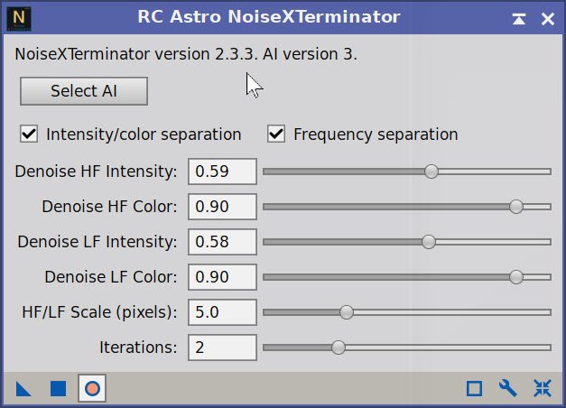
The NXT V3 parameters used.


The Master RGB Image before BXT, After BXT Correction only, After SPCC, After BXT Full Correction, and After NXT=0.7
RGB Stars Image resulting from STX. (click to enlarge)
Master RGB Starless Image after STX (click to enlarge)
5. Process the Linear Lum Image
Run DBE
Start with the RGB sampling plan and then enhance
Use subtraction.
Run BXT Correct Only
Run PFSImage to get star sizes. X = 3.9 , Y= 3.8
Experiment with BXT settings for best results.
Run BXT Full using the star size of 6.8. Much higher than PFSImage star size. See the panel shot below.
Apply NXT - see the NXT Panel snap below.
Take each image starless with STX - use large sample box - no need to save the stars.
Final Master_L sampling plan.
Mastr Lum Before DBE (click to enlarge)
Master_L after DBE. (click to enlarge)
Master_L background removed. (click to enlarge)

PFSImage results for Master L

Final BXT Params used.

Params used with NXT V3.


Master Lum Before BXT, After BXT Correct Only, and NXT v3
Master_L before Star Removal (click to enlarge)
Master L Starless. (click to enlarge)
6. Move Images to the Nonlinear State
For RGB Stars, use HT to adjust with STF disabled until I like the resulting star field.
For RGB Starless, use the current STF->HT method to go nonlinear.
For the Lum image, use the current STF->HT method to go nonlinear.
With starless imaging, I can be much more relaxed about my nonlinear conversion as I can more easily protect my stars from being blown out!
Initial Nonlinear RGB Stars Image (click to enlarge)
Initial Nonlinear RGB Starless image (click to enlarge)
Initial nonlinear Lum Starless Image (click to enlarge)
7. Process the Nonlinear RGB Stars Image
All I am going to do here is use the CT tool to adjust brightness and Saturation until I am happy. Here is the final result.
Final RGB Stars Image (click to enlarge)
9. Do the Processing of the Nonlinear Lum image
Apply the CT to get a nice starting contrast.
Create a Lum_mask by dragging the lum image and making a copy.
Apply the Lum_Mask and then do an HDRMT with level 6 to slightly unblock the highlights - the mask prevents changes to the background.
Do an MLT sharpen with the Lum mask in place (see panel screen snap for parameters)
Apply CT with lum_mask to adjust the tone scale for just the galaxies.
Do an NXT with the V3 parameters shown in the panel snapshot below.
The Initial Lum image (click to enlarge)
Lum_mask Image
After Sharpening with Lum Mask (click to enlarge)
After CT with lum_mask (click to enlarge)
Apply CT (Click to enlarge)
After HDRMT level with Lum Mask(click to enlarge)

Params used in sharpening step
Parameters used in the last NXT V3.


Before and After NXT V3 Application

Final version of the nL_starless image.
10. Complete the Processing of the RGB Starless Image
Apply CT to adjust contrast and saturation.
Apply HDRMT with levels = 6 to open up the highlights
Apply the lum_mask and then apply LHE with a scale of 35, a contrast limit of 2.0, an Amount of 0.7, and an 8-bit histogram.
Run ColorSaturation with the curve shown in the panel snap below.
Apply CT to tweak the tonescale
Using ChannelCombination in CIE Lab mode and just enabling the L layer. Use this to field the Lum image into the RGB Image
Apply CT to adjust the tonescale on the now combined image
Use NXT V3 to lower noise. See the panel shot for the parameters used.
Initial RGB Starles image (click to enlarge)
After HDMRT with levels = 6 (click to enlarge)
After ColorSaturation Adjustment (click to enlarge)
After CT (click to enlarge)
Use CT to tweak the now combined LRGB image (click to enlarge)
After CT (click to enlarge)

After LHE with the lum_msk applied(click to enlare)
Color Sat adjustments done (click to enlarge)
After Lum image insertion (click to enlarge)

NXT V3 params used.


Before and After NXT V3
Final LRGB Starless Image
11. Process the RGB Stars
Apply CT to adjust brightness and color saturation.
Apply SCNR Green a 1.0 to remove some greenish noise seen
Initial nonlinear RGB Stars (click to enlarge)
After CT (click to enlarge)

The Final RGB Star image
12. Combine the RGB Starless with the RGB Stars Image
Use the ScreenStars script to add the RGB Stars back in
The RGB Stars Image (click to enlarge)
The Final Starless LRGB image (click to enlarge)

ScreenStars Panel.

The image with RGB Stars inserted!
14. Export the Image to Photoshop for Polishing
I am pretty happy with the image and ready to polish it in Photoshop.
Save the image as a TIFF 16-bit unsigned and move to Photoshop
Make final global adjustments with Clarify, Curves, and the Color Mixer
Select some feature areas with a lasso with a 100-pixel feather, and use clarity to tweak selected detail areas.
I did the final rotate and crop operation.
I noticed that I had some color rings in the brighter elliptical galaxies. This must be an artifact of the Lu insertion operation, and then boosting the color. I selected these galaxies with the lasso and changed the color mix to make them blend in better.
Added Watermarks
Export Clear, Watermarked, and Web-sized jpegs.

The Final Image!