
Messier 106 - First Light for The Sharpstar SCA260 V2! (10 hours in LHaRGB)
Date: May 17, 2025
Update 5-18-25 - Found the problem with Ha background! See below.
Cosgrove’s Cosmos Catalog ➤#0136

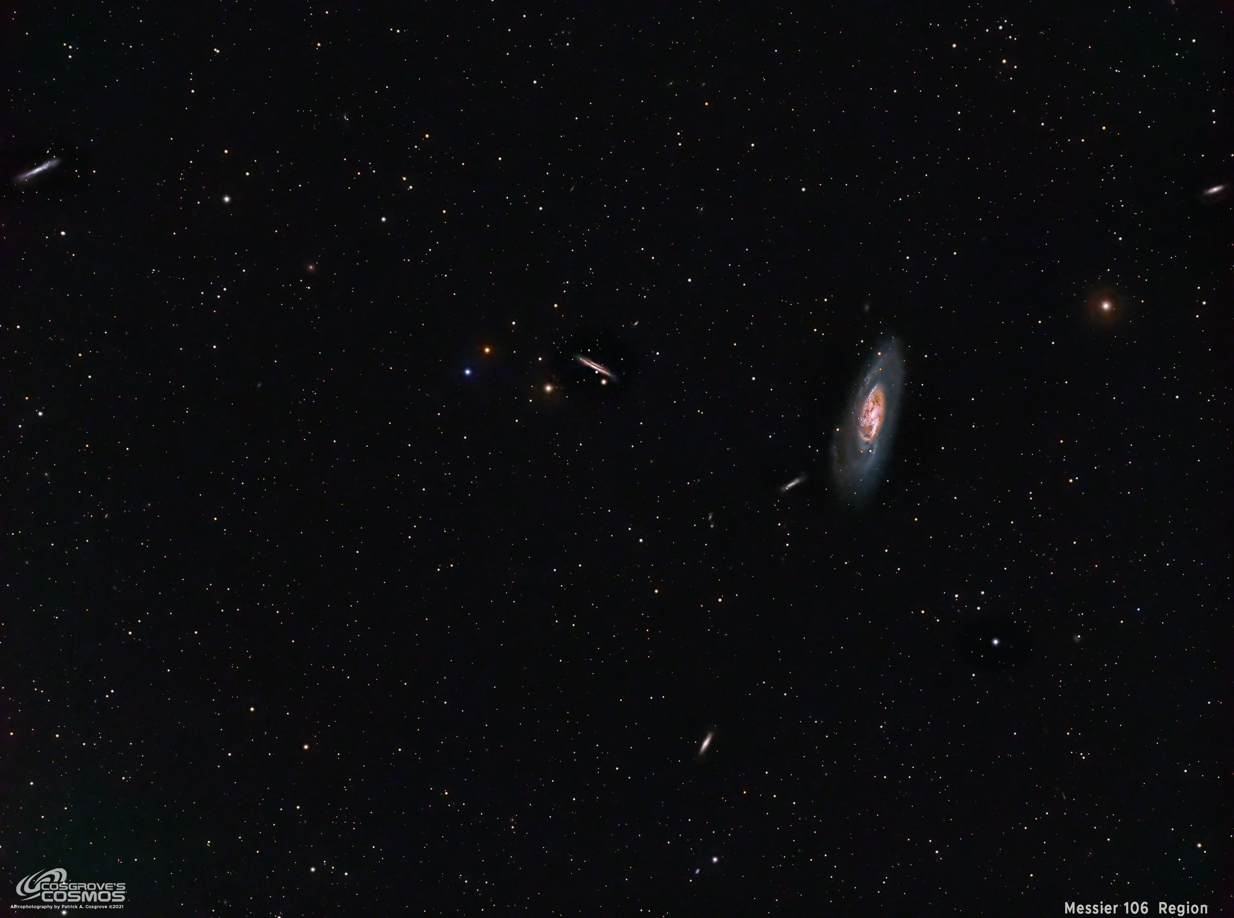
First light for both the Sharpstar SCA260 V2 and the Whispering Skies Observatory! (clck for access to full res image via Astrobin.com)
Chosen for Flickr “Explore” Status, May 17,2025

Table of Contents Show (Click on lines to navigate)
First Light!
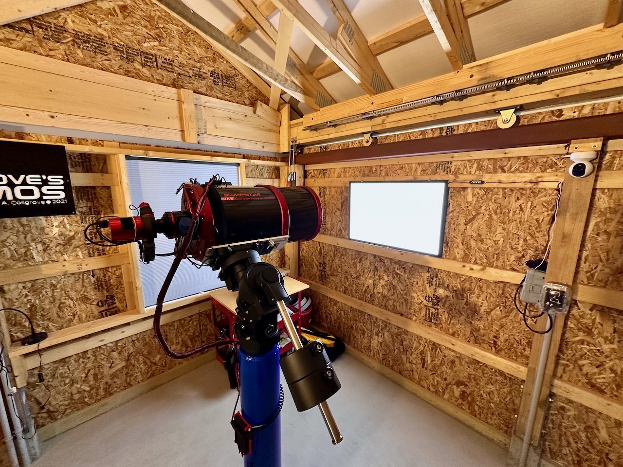
Observatory
After years of effort, my Whispering Skies Observatory project is complete and now operational!
Since construction was finished, I have had two moonless clear nights, and all four telescopes collected photons for the first time!
It’s been over a year and a half since I have had more than one scope in on the action. I must say that it felt really good!
The observatory worked wonderfully, but the telescopes had some issues. It was a maiden cruise with a new setup, computers, and controlling software, so I did run into some heavy seas at times.
Drone view of the Whispering Skies Observatory (click to enlarge)
Telescope
My newest scope, which I placed on my 4th Pier, is the Sharpstar SCA260 V2 Astrograph.
This Super Cassegrain, with a focal length of 1300mm and an f/ratio of f/5, will be my new “Galaxy” scope, and I was eager to see what it could do.
So this imaging project was also the first light for this scope as well!
While I collected data with all four scopes in the observatory, I chose to process this data set first!
The new Sharpstar SCA260 V2 (click to enlarge)
About the Target
Messier 106 (M106), also cataloged as NGC 4258, is a fascinating spiral galaxy located approximately 22 to 25 million light-years away in the constellation Canes Venatici. With a visual magnitude of around 8.4, it is bright enough to be seen with small telescopes and is a favorite target for amateur and professional astronomers alike. M106 spans about 80,000 light-years, making it somewhat smaller than our own Milky Way, but it is remarkable for reasons that go far beyond its size.
One of the most intriguing aspects of M106 is its active galactic nucleus. At its core lies a supermassive black hole actively feeding on surrounding material. This process emits intense radiation and has created unusual features known as “anomalous arms”—jets of hot gas that don’t follow the typical spiral structure seen in most galaxies. These features are visible in radio and X-ray wavelengths, making M106 a significant object of study in understanding galactic evolution and supermassive black holes.

Anomalous Arms. Credit: X-ray: NASA/CXC/Univ. of Maryland/A.S. Wilson et al.; Optical: Palomar Observatory. DSS; IR:NASA/JPL-Caltech; VLA: NRAO/AUI/NSFmolus A
Also visible in this region is NGC 4248, a much smaller dwarf galaxy gravitationally bound to M106. This companion galaxy provides insight into how larger galaxies interact with their smaller neighbors—relationships that often result in gravitational distortions and bursts of new star formation.

Size comparison of our galaxy, M106, and its companion NGC 4248.
Historically, M106 was discovered by Pierre Méchain in 1781, a frequent collaborator of Charles Messier. Despite being a prominent galaxy, it wasn’t officially added to the Messier catalog until much later, during a revision of the list.

M106 was discovered by Pierre Méchain in 178i.

Charles Messier
Its complex structure and active core have since made it a valuable subject for both optical and radio astronomy research.
In this image, you’re not just looking at a beautiful spiral galaxy, but also witnessing cosmic forces at work—gravity shaping galaxies, black holes influencing their environments, and the ongoing processes of stellar birth and death.
Annotated Image

Image created with Pixinsight’s ImageSolver and AnnotateImage scripts.
Location in the Sky

Findershart created with Pixinsight’s ImageSolver and FinderChart scripts.
About the Project
Typically, I spend a great deal of time researching my targets and preparing for a night of capture.
This time, not so much.
I was swamped trying to get everything set up in the observatory. I had four new Mele Quiter 4C microcomputers to configure, all of which would use NINA software. While I had learned to use NINA on my FRA400, I now had to reinstall it on a new computer for that platform and get it set up and operational while getting the other three platforms up for the first time.
In addition, I had just finished putting together the SCA260 platform, which was going to be used for the first time.
There were a thousand details that had to be configured just so.
I was a bit distracted.
So I cheated. I used ChatGPT to plan out a list of targets. It seemed to do an amazing job. (Once I process and write up the imaging projects for the other scopes, you will learn all about trying to shoot targets that were actually well below the horizon - but not according to Chat GPT!).
Anyhow, on that list was M106. I have shot this target before, so I was familiar with it. I thought it might be a good target for the maiden voyage of this scope.
It’s not overly large as galaxies go, but it was not tiny either. It also had some interesting details. So, I decided to choose this target and capture it in LRGB, along with some Ha data.
With my plan in place, I set up NNA to go after it.
Previous Efforts
I first shot M106 back in May of 2020. It was a very short integration of only 1.3 hours in LRGB. This was shot with my William Optics 132mm platform. You can see the Imaging project post for that early effort HERE. That image can be seen below:

My first effort shooting M106 back in 2020 with an integration of only 1.3 hours.
My second effort involving M106 was done in June of 2022. This time I was using the FRA400 platform and was dealing with a wide field view of the region. This was a 5.7 hour LRGB integration. The post for that project can be seen HERE. That image can be seen below.
My second M106 effort was a 5.7 hour LRGB integration shot with the FRA400 platform.
Both of these efforts suggest the detail apparent in M106, so it would be very interesting to see what could be done with the new SCA260 platform.
Data Capture
On April 22, we had the first clear, Moonless night since I had the telescope gear installed in the observatory.
Before I could start my session with the SCA260, I wanted to do a focus offset series with NINA. This would determine the focus position of each filter relative to the Lum filter. With this in hand, I could create a very efficient series where I could capture Ha, L, R, G, and B filter subs, one after another, without having to do a focus series with the filter change. This provides a balanced collection of subs, so if the weather shuts me down, I have a set I could process.
Once it got dark enough to see the stars, I kicked off the process in NINA to do that. This took about 2 hours to finish. Once that was done, I started capturing data.
I had never guided with an OAG rig before, nor had I ever used the IOptron CEM70 mount - so I had to watch to see how they did.
I was unsure if this was a good idea, but I left the fans on to circulate air on the back of the SCA260 mirror during the exposures. I had seen a recommendation to do this online. The advantages here are that it helps the mirror acclimate to the ambient temperatures, and it is also helpful in preventing DEW. Reports suggested that the SCA260 was a DEW magnet, so I went with it. In the future, I plan on doing a rigorous test to see if running the fans impacts image sharpness. But for this outing, I would leave them on.
Since I started late, M016 was pretty high in the sky. I was watching the tracking on PHD2, and I have to say - things were looking ugly here. I did not understand why it looked as bad as it did! My experience with the CEM60 has been wonderful.
Then I started to hear some strange sounds from the mount! This can’t be good.
I turned on my red headlamp and went to investigate.
I discovered my first bonehead move of the project. I had never set up a Meridian flip, and it was past due! I killed the session, did a manual meridian flip and stated things off again.
Now, on the other side of the pier, tracking looked much better, running an average of about 0.6 RMS. So I let things run.
I checked a while later and found that while the tracking was looking good, every once in a while, I would see a spike that should not be there. This was concerning and something that I would have to investigate later.
After the rough start, the platform seemed to be working well for the remainder of the evening. I shut things down before twilight, satisfied that I had a good start.
The next day, I installed blackout drapes on the observatory and shot all of my calibration frames.
For the flats, I bought an A1-sized LED tracking panel and mounted it on the wall adjacent to the SCA260. I simply had to park the scope to point it at the panel and then I could use the Flatwizard on NINA to capture my flats. Easy Peasy.
My Flats set up for the SCA260.
Well, not quite.
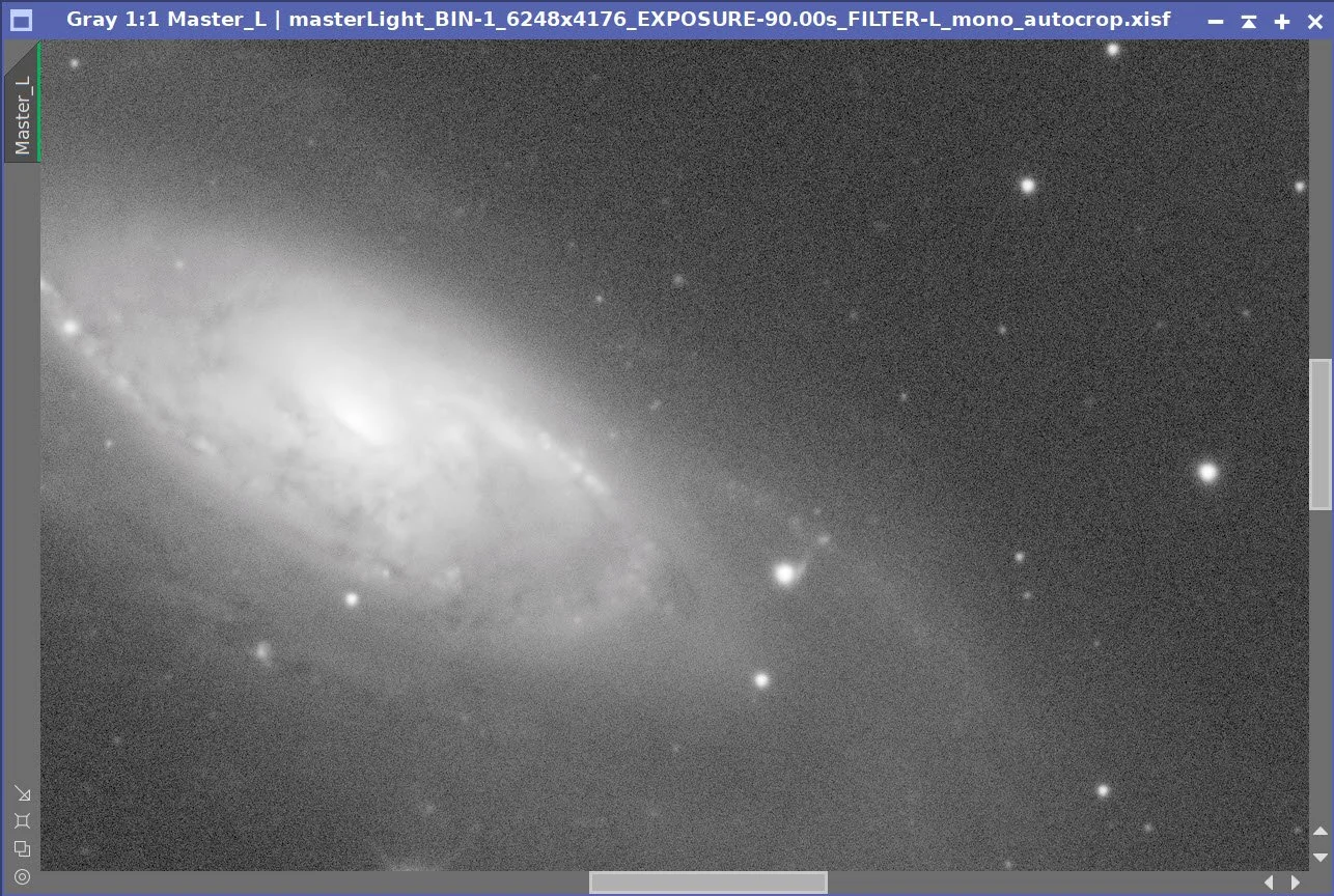
I tried processing the Lum data from the previous night with NO Flats to see how things looked. I found this:

Lum data from the first night - NO FLATs calibration.
Not too surprising. Vignetting. Dust. I certainly need those Flats!
So I looked at the flats:
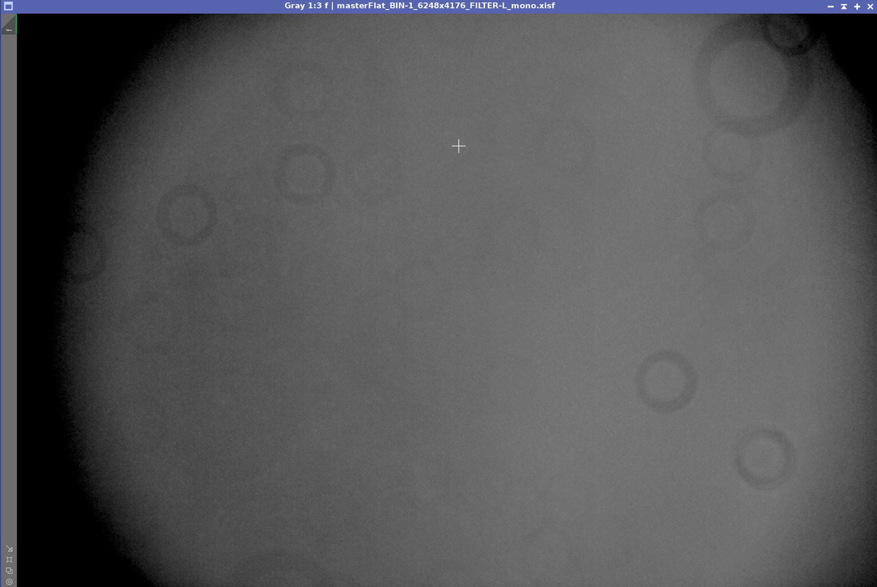
My Lum flat master.
These, as expected, looked like they should.
So I reran WBPP with all the cal data for the Lum subs I had so far, and got this:

Master Lum after adding cal files to WBPP.
Wait - WHAT? My dark vignetting is now light vignetting! My dark dust rings are now light dust rings!
My Flats were overcorrecting! It took me a long time to figure out what was going on. I have been using flats for years with no issues, and now suddenly, it's a big issue!
I finally found the cause and corrected the problem. Rather than discuss that here, I have created a separate post on the problem, which you can see HERE.
The next clear night was on the 27th, and I must say that after a rough start on the first night, the second night ran like clockwork!
After collecting all of this data, I could not wait to process it! But wait, I must, as I was going to be out of town for almost two weeks, so I had to come back to it later.
Image Processing
After reviewing all of the subs in Blink, I found that there were periods during the second night when some thin clouds came in, so I ended up removing more subs than I would like.
I also saw a handful where the tracking was bad. This seems to correspond to the spikes I had seen in the PHD tracks. I took a look at the PHD logs, and it seems that at least part of the problem was guide stars losing mass or having a poor SNR. I am new to OAG, so there is more I may need to do there. I also have to see if my 3D balance is good and whether there are positions where cable drag could be an issue.
After correcting my flat's problem, the correction seemed much better, but I did see some residual rings in one corner that had an ‘embossed” look. This is typically created what the filter positioning is not consistent. I may need to rerun the EFW calibration to help with this for future efforts.

“Embossed” Rigs - a residual from flat calibration indicating filter positioning errors.
The other thing I found was that the Master Ha image had a dark nonuniformity in the center of the field and a linear mark to the side. I believe this was caused by the LED panel I used as a flat source.
I found this pattern in ALL of my master images. It was very subtle in my LRGB images, while in the Ha image, it was quite pronounced, as you see below. Some of this is caused by the Screen stretch applied - when I explored the change in values over this region, they are quite small.
UPDATE!!
〰️
UPDATE!! 〰️
I found the source of this pattern in the Ha data. I went over every bit of data again, expecting to find a problem with my Flats Panel.
I could NOT find this pattern at all in the raw lights.
I could NOT find this pattern at all in the raw Flats
I could NOT find this pattern at all in the raw Flat Darks
I could NOT find this pattern at all in the MasterFlats!
So I looked again at my 300 seconds darks.
And there - I saw it!
It was very subtle. But once I spotted it, I could not miss it.
It would appear that I have a light leak in the optical system.
I saw the problem most pronounced in the Ha. It was also present for LRGB but at a lower magnitude.
This makes sense:
The LRGB exposure was 90 seconds, and the darks were exposed for 90 seconds to a small light leak.
The Ha exposure was 300 seconds. So those darks had a longer exposure to the light leak.
When I shot these, I had some dark plastic over the windows, making the observatory dark, but not super dark.
I will have to reshoot these at night.
The good news is that my LED panel is working fine!
I am glad to have found this and am able to update the posting for this project to let you know!
Now back to the post!

Non-uniformities in the Master Ha image!
I tried to minimize this using DBE, but it only went so far.
This is a shame, as the Ha image is really interesting. It clearly shows the anomalous arms that are somewhat unique to this galaxy.

Anomolous Arms seen in the Ha image!
I did manage to incorporate some of the Ha Starless data into the final image, but the effect is probably more subtle than I would like.

A zoomed in view of the final image. The anomolous arms can be seen at about 10-11 O’clock, relative to the core.

Zoomed in even further.
On another front, I did something different for star sizes.
In the past, I feel I have been guilty of using BXT to reduce the size of the stars and may have gone too far at times. So, this time around, I was conscious of not reducing my star sizes too much, so they are larger and have more color. In addition, since stars from this scope have defraction spikes, I adjusted the intensity of the stars to show these in a way I thought was pleasing.
I may have gone too far on this - so I will see what feedback I get on the image.
Other than that, the image processing was straightforward.
Results
In general, I am pleased with the quality of this first image. It shows the promise of the SCA260, while still pointing out where I have issues that I need to resolve, which include:
Determining if the collimation is optimal
CEM70 tracking spikes
Fine-tuning the OAG PHD2 guiding
Issues with my LED Tracing panel light source
I think the collimation is pretty good, and that is a testament to the scope's design and how well it was packaged. It shipped from China to the Western US and then across the country to Upstate NY. Despite this worldwide travel, I have not needed to change the centering of the secondary mirror, and the primary mirror is good enough that my stars are reasonably formed.
At some point, I will get my hands on a Howie Glatter laser and resolve the lingering questions about collimation.
Another comment I will make is how rusty I felt doing the LRGB processing here!
Since the move and construction of the observatory, my shooting has been very limited, and most of it has been dealing with narrowband images.. But it is slowly coming back to me.
Finally, I was super stoked to see that I had captured the Anomalous Arms in my Ha data—that is so cool! However, the fact that I had nonlinearities in the flats compromised the best way I had to integrate that data with the LRGB, so I don’t think I did the best job here.
This feels like a target I will revisit—perhaps adding more data once my Ha flats issues are resolved!
More Info
🔭 General Information
Wikipedia – Messier 106
Comprehensive overview including discovery, structure, and significance.
NASA Science – Messier 106
Detailed insights from NASA’s Hubble mission, featuring images and scientific context.
🌌 Imagery and Visual Resources
ESA/Hubble – Hubble View of Messier 106
High-resolution images combining Hubble data with amateur observations.
NASA HubbleSite – Galaxy M106
Close-up imagery and details about M106’s structure and features.
NASA Chandra X-ray Observatory – NGC 4258 (M106)
X-ray observations revealing the energetic processes at M106’s core.
🧪 Scientific Studies and Articles
Spitzer Space Telescope – Mystery Spiral Arms Explained
Discussion on the anomalous arms of M106 observed in different wavelengths.
Astronomy Picture of the Day – M106: A Spiral Galaxy with a Strange Center
Daily astronomical image featuring M106 with explanatory notes.
🧭 Additional Resource
Constellation Guide – Messier 106 (NGC 4258)
Information on M106’s location within the constellation Canes Venatici.
NASA Scientific Visualization Studio – Spiral Galaxy M106
Visualizations and animations depicting M106’s structure and dynamics.
Capture Details
Lights
Number of frames is after bad or questionable frames were culled.
72 x 90 seconds, bin 1x1 @ -15C, unity gain, ZWO Gen II L Filter
82 x 90 seconds, bin 1x1 @ -15C, 0 gain, ZWO Gen II R Filter
76 x 90 seconds, bin 1x1 @ -15C, unity gain, ZWO Gen II G Filter
73 x 90 seconds, bin 1x1 @ -15C, unity gain, ZWO Gen II B Filter
29x 300 seconds, bin 1x1 @ -15C, unity gain, Astronomiks 6nm Ha Filter
Total of 10 hours 7 minutes
Cal Frames
30 Darks at 300 seconds, bin 1x1, -15C, gain 0
30 Darks at 90 seconds, bin 1x1, -15C, gain 0
30 Dark Flats at each Flat exposure times, bin 1x1, -15C, gain 0
15 R Flats
15 G Flats
15 B Flats
15 L Flats
15 Ha Flats
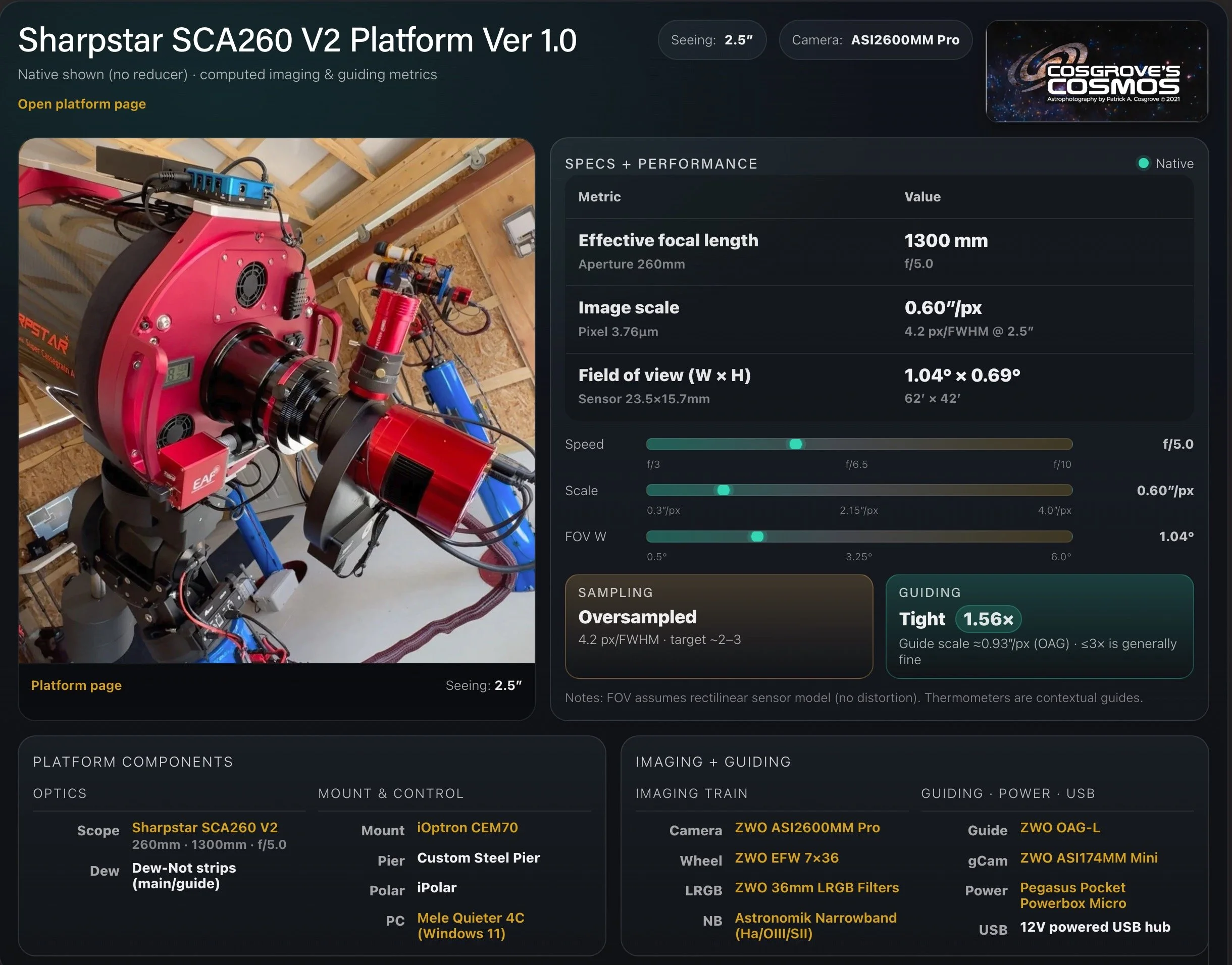
Platform used for this project
Software:
Capture Software: PHD2 Guider, NINA
Image Processing: Pixinsight, Photoshop - assisted by Coffee, extensive processing indecision and second-guessing, editor regret and much swearing…..
Image Processing Detail (Note: This is all mostly based on Pixinsight)
1. Assess all captures with Blink
Light images
Lum images:
Removed 3 - tracking issues
Removed 2 - thin clouds
Red images:
Removed 3 for tracking
Removed 5 for clouds
Green Images:
Removed 1 for tracking
Removed 2 for clouds
Blue Images:
Removed 3 for tracking
Removed 6 for clouds
Ha Images:
Removed 3 for clouds
Flat Frames - no issues seen on individual subs
Flat Darks - no issues seen
Darks - no issues seen.
Summary:
37.5 minutes lost to clouds
15 minutes due to tracking.
Not a big deal - but I rarely lose subs to tracking so I definitely have an issue to resolve here!
2. WBPP Script
Load all files
Dark exp tolerance set to zero
Light exp tolerance set to zero
Pedestal auto for all frames
CC auto for all groups
Select max quality
Ref image set to auto
Selected the target folder
Executed in 1:15 with no errors

WBPP setup.

Post Processing View of WBPP

WBPP Pipeline view
3. Import Master images and Rename

Master images. Top: Lum and Ha. Bottom: Red, Green, and Blue.
Note that all of the frame show some nonlinearities - the work being with the Ha Master. Clearly, I need to work on my flat light source!
4. Create and Process the RGB Color Image
Create the Master_RGB image using the ChannelCombination Tool
Apply DBE to remove the gradient and nonuniformities seen.
Apply BXT on the color image with “Correct Only”
Run SPCC
Apply BXT with full correction. See panel-snap for values used.
Since this color image will be processed for color and low noise, I went a bit light on the BXT restoration. I will go heavier on the Lum image, which will be processed for sharpness and detail.
Run NXT = 0.45
Run STX to go starless. Preserve the stars and use the unscreen technique

The initial Master_RGB Image
DBE Sample pattern for RGB image. (click to enlarge)
RGB image before DBE. (click to enlarge)
RGB image after DBE. (click to enlarge)
Background image subtracted. (click to enlarge)

The setup used for SPCC.
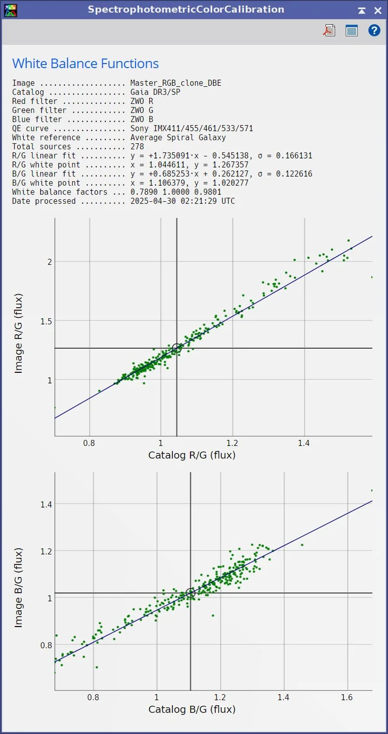
The correlation found.
Before SPCC. (Click to enlarge)
After SPCC. 9Click to enlarge)

BXT settings used. Determined by trial. A bit on the light side for color image.


RGB Image Before BXT, After BXT Crorrect Only, After BXT Full Correction, After NXT=0.45
Master_RGB_Stars (click to enlarge)
Master_RGB_Starless (click to enlarge)
5. Process the Lum Image
Using a sampling pattern similar to the RGB plan, customize and run DBE.
Run BXT Fix only.
Run PFSImage and get the FWHMx= 4.25, FWHMy = 4.08
Run BXT full - using the panel value shown below.
Run NXT= 0.55
Master Lum sampling Plan
Lum image before DBE (click to enlarge)
Lum image after DBE (click to enlarge)
Lum background imae subtracted. (click to enlarge)

The PFSImage Panel used to get the FWHM measures.

The values used for BXT.


Lum Before BXT, After BXT Correct Only, After BXT Full Correction, After NXT=0.55
Lum Starless. (click to enlarge)
Lum Stars only - not used. (click to enlarge)
6. Process the Ha Image
Run DBE and attempt to correct for the problematic nonuniformity. (See update at front of post - I found the cause of this!)
Create an aggressive sampling pattern around problem areas and run DBE.
Run a second time to minimize the problem
Run BXT Correct only
Run PFSIMage. FWHMx = 4.93, FWHMy= 4.83
Run Full BXT using the parameters shown in the panel snapshot below.
Run NXT = 0.55
Subtract stars using STXpreserving the RGB stars
Ha sampling Plan for DBE (click to enlarge)
2n- same pattern. (click to enlarge)
Ha before DBE (click to enlarge)
Where we are now. (click to enlarge)
Ha after DBE (click to enlarge)
New result - far from perfect!
Ha DBE Backgrond removed (click to enlarge)
2nd Background. (click to enlarge)
After two runs, it is better but far from perfect. I will have to try to bury the problem into the background.

PFSImage run for Ha

Parameters used for BXT on Ha.


Ha Image Before BXT, After BXT Correct Only, After BXT Full Correction, After NXT=0.5
Master Ha Starless - note the problematic background.
7. Take Images Nonlinear
For the Starless images, use the STF->HT method to go starless.
For the RGB Star images, I used HT to stretch the image to the point where I liked the star sizes. Note that in the past I think I went too small on stars to this time around I am going to try for larger stars with more color.
Nonlinear Lum (click to enlarge)
Nonlinear Ha - with crummy background! (click to enlarge)
Nonlinear RGB (click to enlarge)
Nonlinear RGB Stars (click to enlarge)
8. Process the Nonlinear Lum Starless Image
We want this image to be very sharp and detail-oriented. We also want it to be a little on the dark side to prepare it for injection into the RGB image.
Apply a CT to do an initial shape of the tone scale
Run LHE with a Scale of 170, a Contrast limit of 2.0, an Amount of 0.25, and use a 10-bit histogram
This adjusts the large-scale feature contrast.
Apply another CT to shape the result a bit.
Run the DarkstructuresEnhance script with default parameters.
Then, I did another LHE with parameters scale 64, a Contrast Limit of 2.0, an Amount of 0.16, and an 8-bit histogram.
This is to adjust the contrast of smaller-scale features.
Finally, let run NXT and use some of the features of the new version 3.0 model:
color_separation = false;
requency_separation = True;
denoise = 0.70
denoise_color = 0.90;
denoise_lf = 0.9;
denoise_lf_color = 0.9;
requency_scale = 5.0;
.iterations = 2;
detail = 0.15;
Note: I will zoom in a bit on the images below so you can get a better feel for the detail being revealed.
The initial Lum nonlinear Starless image. (click to enlarge)
After CT adjust (click to enlarge)

Lum after LHE1 - Large scale feature contrast (click to enlarge)
After LHE2 - Small Feature Contrast Adjust. (click to enlarge)
After DarkStructureEnhance script(click to enlarge)
After NXT with new Ver 3 model params as documented in the text (click to enlarge)

A CT complete the final Lum Starless Image.
9. Process the Nonlinear Ha Starless image
Use CT to drop out the background and focus on key Ha features.
Use GAME to create a gradient mask that covers M106 and its companion
Apply the mask and invert it so you are dealing with the background
Now apply CT to drop it out.
Apply LHE with params: Scale 20, Contrast Limit 2.0, Amount 0.4, 8-bit histogram, with Ha_Mask applied
Apply CT with HA_Mask applied
Now run NXT V3 with these params:
P.enable_color_separation = false;
P.enable_frequency_separation = true;
P.denoise = 0.90;
P.denoise_color = 0.90;
P.denoise_lf = 0.5;
P.denoise_lf_color = 0.9;
P.frequency_scale = 5.0;
P.iterations = 2;
P.detail = 0.15;
Do a Final CT
The initial nonlinear Ha image (Click to enlarge)
Tonescale adjust with CT to drop out backlground. (Click to enlarge)
IHa_Mask (click to enlarge)

After LHE for small scale detail (click to enlarge)
NXT with V3 Paramters
After CT with ~Ha_Mask (click to enlarge)
After CT with HA_Mask

10. Process the RGB Image
The goal here is first to create a high-color, low-noise image that is a bit on the dark side in preparation for integrating Lum data into the RGB data.
Create WarmMask
Use ColorMask_Mod script with a starting hue of 350 and an End hue of 60
Boost with CT
Blur with Bill Blanshan’s Blur Script
Create CoolMask
Use ColorMask_Mod script with a starting hue of 166 and an end hue of 264
Boost with CT
Blur with Bill Blanshan’s Blur Script
CT to boost contrast and color Sat
Apply LHE with params: Scale 64, Contrast Limit 2.0, Amount 0.14, and an 8-bit histogram to enhance small-scale detail.
Apply WarmMask and CT to adjust intensity and Sat
Apply CoolMask and CT to adjust intensity and Sat
Do a final CT to darken things a bit before doing the Lum insertion
Use the ChannelCombination tool with CIE color and only the Lum selected to fold Lum data into RGB
Do a CT to adjust things.
Use PixelMath with the equation shown and $T[1] for green and $T[2] for blue, AND the Ha-Mask to add Ha contribution to RGB
Use the Ha_Mask and CT to correct the color balance of the galaxy core after adding Ha.
Create the WarmMask:
Seetings for creating WarmMask. (click to enlarge)
Initial WarmMask. (click to enlarge)
Apply CT to boost. (click to enlarge)

WarmMask afer blurring.
Create CoolMask:

Initial CoolMask. (click to enlarge)
CoolMask after CT Boost (click to enlarge)
CoolMask after Blur
Now, lets process the RGB image. I will use a zoomed in view here so that you can better see what is going on.
Initil RGB Starless Image (clcik to enlarge)
After Small scale detail LHE (click to enlarge)
CT with CoolMask (click to enlarge)
Use Channel Combnation Tool to insert Lum data into RGB. *click to enalrge)

Primary PixelMath Expression to add Ha to red.
Ha_Mask - create with GAME, used to focus on the galaxies and correct the color balance
After initial CT (Click to enlarge)
CT with WarmMask (click to enlarge)

CT Adjust (click to enlarge)
CT to do a final ddjust (click to enlarge)
Ha data Added (Click to enlarge)

CT curve used to fix balance
CT with the Ha_Mask to create teh final RGB Starless Image (click to enlarge)
11. Process the RGB Stars
Use CT to adjust the tone scale and color saturation to create the final look for the image.
Choose the medium level of stars for the final image. The large was too much, but the medium level showed the stars nicely and had good color.
The initial RGB nonlinear star image.

Using CT, I made the stars much bigger than I normally do so that I could have more color and drama.
11. Add the Stars Back In and Complete Processing
Use the StarScreen script to add the stars back in.
Run NXT using model 3:
P.enable_color_separation = true;
P.enable_frequency_separation = true;
P.denoise = 0.90;
P.denoise_color = 0.90;
P.denoise_lf = 0.5;
P.denoise_lf_color = 0.5;
P.frequency_scale = 5.0;
P.iterations = 2;
P.detail = 0.15;
Crop the image
The Final Starless Image. (click to enlarge)
The Final RGB Stars image. (click to enlarge)
The ScreenStars script combines the stars and starless images.


Before and After the Final NXT

After DarkStructureEnhance.
12. Move to PhotoShop and do the final Polish
Export as 16-bit tiff
Open in Photoshop
Use the Camera Raw filter to tweak color, tone, and Clarity
Use Camera Raw ColorMixer to adjust the blues and orange tones
Add watermarks
Export various versions of the image
The Result!