
Messier 106 Region - 5.7 hours LRGB
Date: June 27, 2022

This image was granted Flickr “Explore” status on 6-28-22!
Cosgrove’s Cosmos Catalog ➤#0103
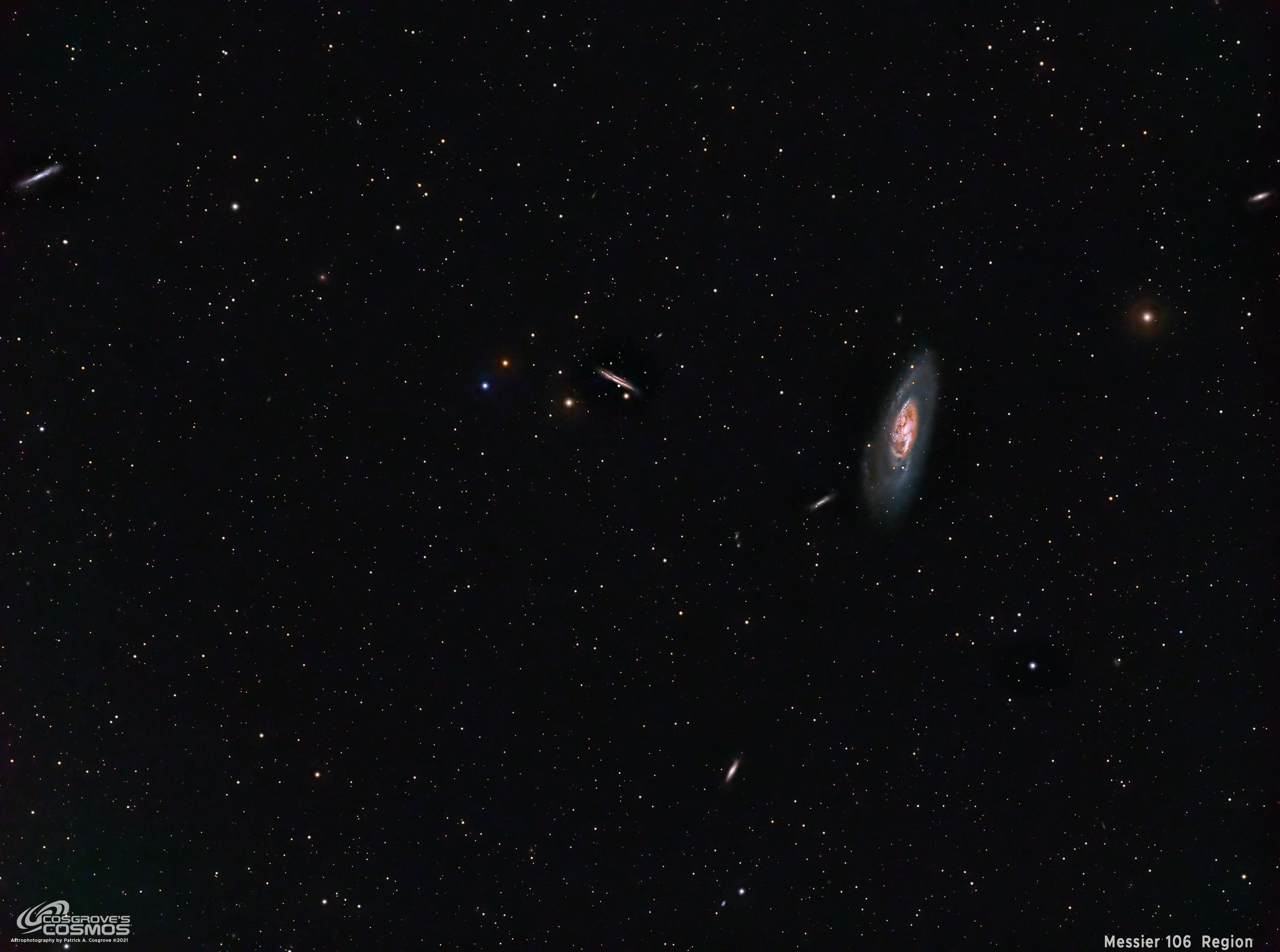
This is about a two degree radius view of the M106 Region - note the number of small galaxies nearby! (click for the full resolution version of the image via Astrobin.com)
Table of Contents Show (Click on lines to navigate)
About the Target
M106, also known as NGC 7353, is a galaxy in the constellation Canes Venatici (The Hunting Dogs), which is located between 22 and 25 million light-years away. M106 is a massive galaxy with a very active core region that is home to a supermassive black hole.
Wikipedia tells us the following about M106:
M106 has a water vapor megamaser (the equivalent of a laser operating in microwave instead of visible light and on a galactic scale) that is seen by the 22-GHz line of ortho-H2O that evidences dense and warm molecular gas. Water masers are useful for observing nuclear accretion disks in active galaxies. The water masers in M106 enabled the first case of a direct measurement of the distance to a galaxy, thereby providing an independent anchor for the cosmic distance ladder. M106 has a slightly warped, thin, almost edge-on Keplerian disc which is on a subparsec scale. It surrounds a central area with mass 4 × 10⁷M⊙.
It is one of the largest and brightest nearby galaxies, similar in size and luminosity to the Andromeda Galaxy. The supermassive black hole at the core has a mass of (3.9±0.1)×107 M☉.
M106 has also played an important role in calibrating the cosmic distance ladder. Before, Cepheid variables from other galaxies could not be used to measure distances since they cover ranges of metallicities different from the Milky Way's. M106 contains Cepheid variables similar to both the metallicities of the Milky Way and other galaxies' Cepheids. By measuring the distance of the Cepheids with metallicities similar to our galaxy, astronomers are able to recalibrate the other Cepheids with different metallicities, a key fundamental step in improving quantification of distances to other galaxies in the universe.
Here is some detail on the other galaxies that can be seen in this image:
NGC 4248 is the edge-on galaxy located adjacent to M106 to the lower left. It is located 25 Million Light years away.
NGC 4217 is an edge-on galaxy with a prominent dust lane located almost directly towards the left of M106. This galaxy is located 60 million light-years away.
NGC 4226 is located towards the top right of NGC 4217. It is a barred spiral galaxy.
NGC 4231 /4232 are a pair of galaxies that can be seen to the lower left of M106.
NGC 4144 is a barred spiral galaxy in the constellation Ursa Major. It was discovered by William Herschel on April 10, 1788. It can be seen on the extreme left side of the image frame.
NGC 4346 is a small lenticular galaxy seen on the extreme right side of the frame.
NGC 4218 is a spiral galaxy that is 34 million light-years away. It can be seen at the very bottom of the frame.
NGC 4220 is a lenticular galaxy, also seen at the bottom of the frame.

This annotated image was created in Pixinsight, using the ImageSolver and Annotate Image Scripts.
The Location in the Sky

This finger chart was created in Pixinsight using the FinderChart process.
About the Project
If you have been following Cosgrove Cosmos, then you know that I run three telescopes each night when I capture subs.
In a region where clouds seem to dominate, my philosophy is to capture as much as you can for as long as you can when you have the opportunity. So I run three scopes in my driveway - in parallel - to capture as many photons as I can.
This can be, however, a challenge during galaxy season.
Two of my scopes are longer focal length refractors with about a 5” diameter. One is 920mm and the other is 1080mm. These provide a reasonable image scale for going after galaxies - well at least the larger ones!
But my third scope is a 72mm diameter astrograph with a focal length of 400mm. I have a wider field of view with this rig - which is great when you are shooting larger nebulous regions. But driving galaxy season? Sometimes I have a really hard time finding a target that is suitable for this image scale.
Target Selection
As I looked for a good target, I could not find anything that I liked. So I decided to look for a field that was rich in galaxies and see what that might look like.
I finally chose the area around Messier 106. I had imaged this galaxy before (we will revisit that effort in a minute), so I was familiar with it. It was also a larger galaxy so I would have at least one galaxy in the field with some detail to it It also had a scattering of galaxies in its general region. So I decided to focus on this region.
Using the Framing and Mosaic tool in SGP, I composed the image to capture a selection of galaxies of various sizes. With this done, I set up my sequence collection plan in SGP and captured LRGB data for the next few nights.
This image was captured over the Nights of 5-29-22, 5-30-22, and 5-31-22.
Previous Effort
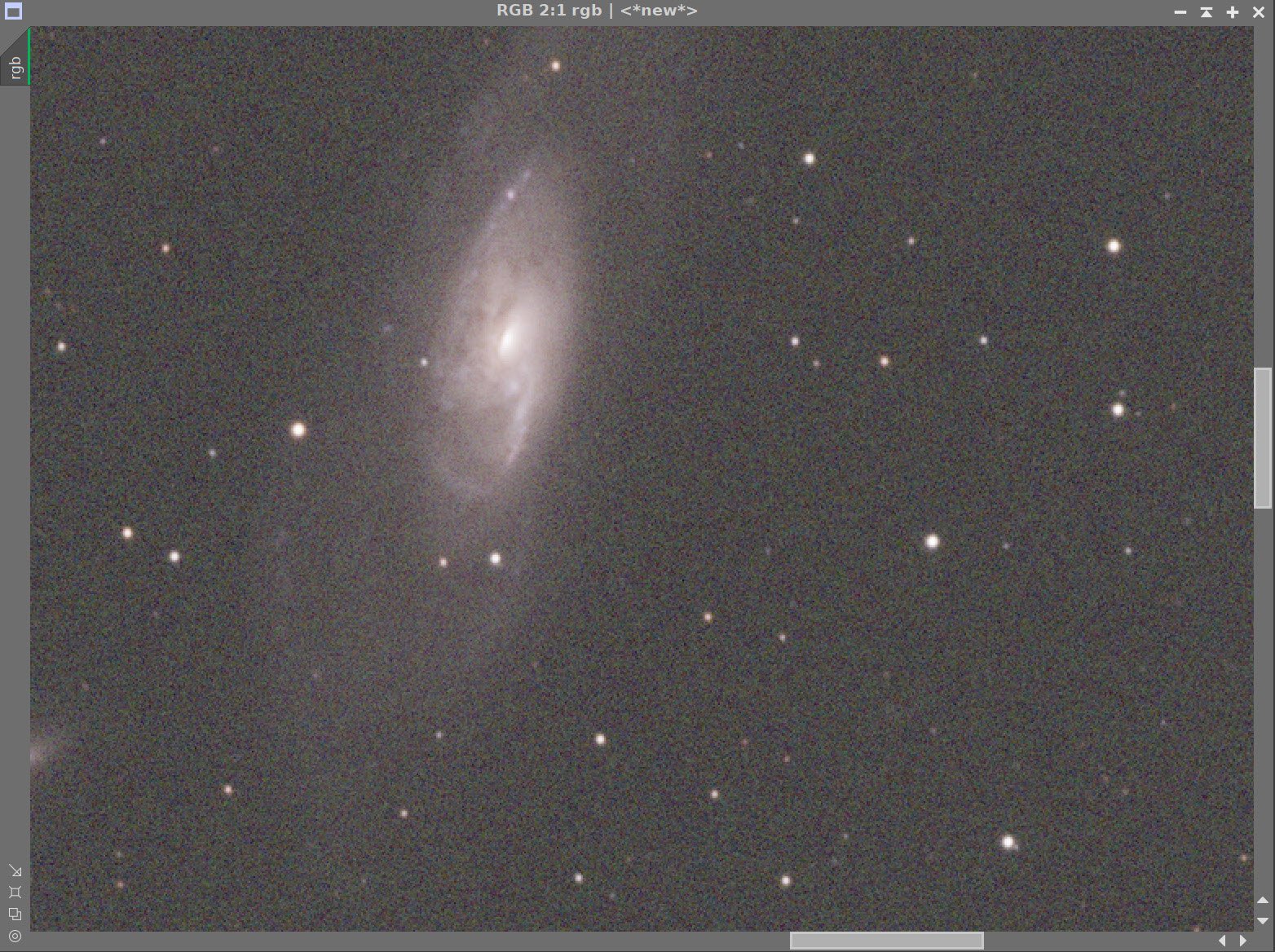
I first shot M106 in May of 2020. The story of this image can be seen HERE.
This was shot with my William Optics 132mm FLT rig using a ZWO ASI294MC-Pro OSC Camera and with 1.3 hours of exposure.
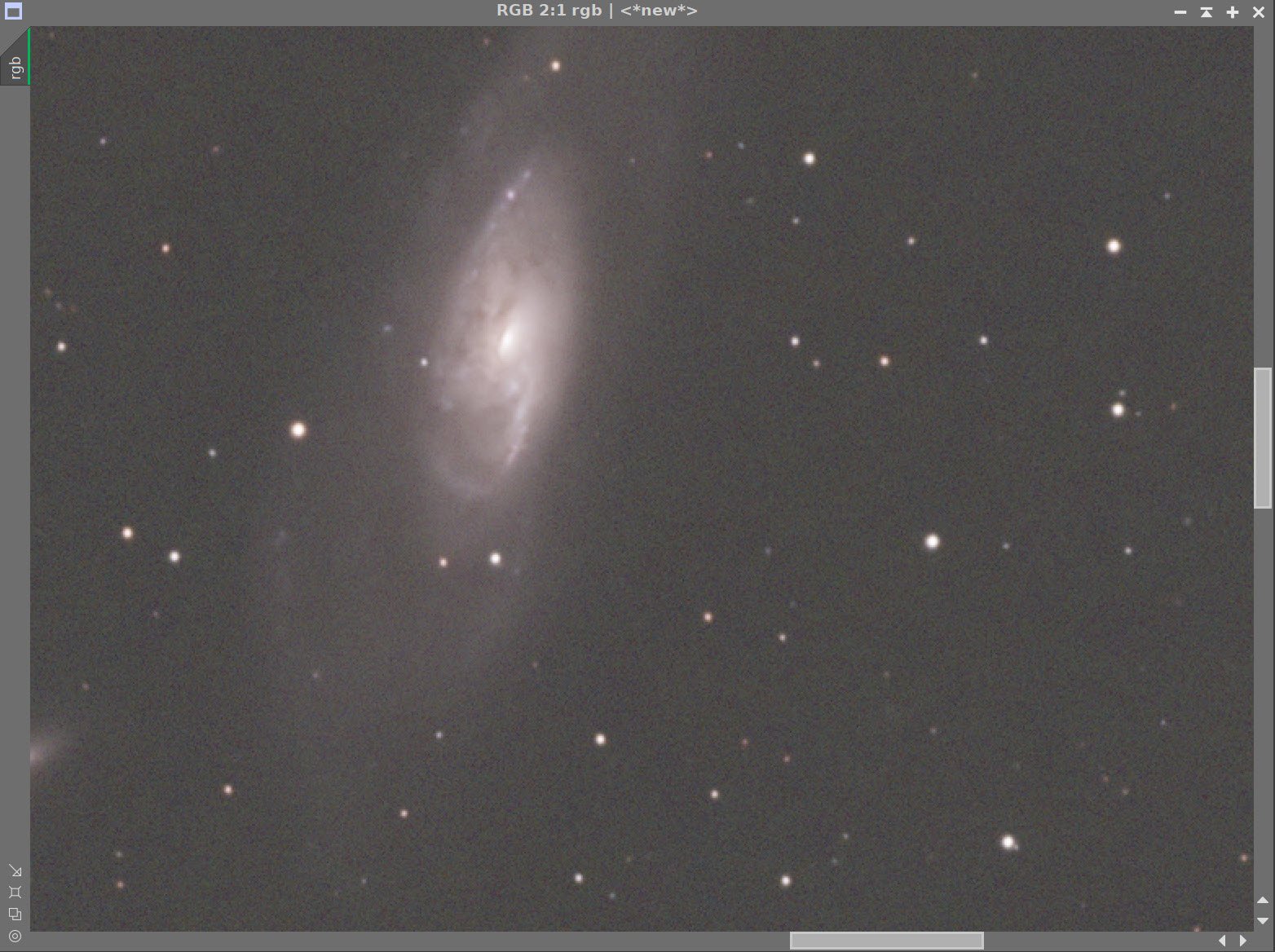
The new image uses my widefield scope and a ZWO ASI1600MM-Pro camera with 5.7 hours of LRGB exposure. You can see the comparison of these two shots below:
This was my effort form May 2020. (click to enlarge)
And here is my current effort. (click to enlarge)
Even though the newer version is smaller, it seems to have superior detail and color compared to my first effort. Seeing this, I am very tempted to revisit this target next year with the Astro-Physics 130mm platform. With its longer focal length and next-generation camera, I have to believe I could get a great result from it!
A detailed Processing Walk-Through is provided for this image at the end of the posting…
More Information
Wikipedia: Messier 106
NASA Hubble Images: Messier 106
BBC Sky At Night: Messier 106
Messier-Objects.com: Messier 106
Capture Details
Lights Frames
Data was collected during the Nights of 5-29-22, 5-30-22, and 5-31-22
46 x 90 seconds, bin 1x1 @ -15C, Gain Unity, ZWO Gen II Lum filter
59 x 90 seconds, bin 1x1 @ -15C, Gain Unity, ZWO Gen II Red filter
57 x 90 seconds, bin 1x1 @ -15C, Gain Unity, ZWO Gen II Green filter
66 x 90 seconds, bin 1x1 @ -15C, Gain Unity, ZWO Gen II Blue filter
Total of 5.6 hours
Cal Frames
25 Darks at 120 seconds, bin 1x1, -15C, gain Unity
25 Dark Flats at Flat exposure times, bin 1x1, -15C, gain unity
12 flats Flats at bin 1x1, -15C, gain unity
Software
Capture Software: PHD2 Guider, Sequence Generator Pro controller
Image Processing: Pixinsight, Photoshop - assisted by Coffee, extensive processing indecision and second-guessing, editor regret, and much swearing…..
Capture Hardware:
Scope: Askar FRA400 73MM F/5.6 Quintuplet Astrograph
Guide Scope: William Optics 50mm
Camera: ZWO ASI1600mm-pro with ZWO Filter wheel with ZWO LRGB filter set, and Astronomiks 6nm Narrowband filter set
Guide Camera: ZWO ASI290Mini
Focus Motor: Pegasus ZWO EAF 5V
Mount: Ioptron CEM 26
Polar Alignment: Ipolar camera
Software:
Capture Software: PHD2 Guider, Sequence Generator Pro controller
Image Processing: Pixinsight, Photoshop - assisted by Coffee, extensive processing indecision and second-guessing, editor regret and much swearing…..
Click below to see the Telescope Platform version used for this image
Image Processing Walk-Through
(All Processing done in Pixinsight - with some final touches done in Photoshop)
1. Blink Screening Process
Lum Images: lots of trails are seen - looks good!
Red: lots of trails are seen - some gradients.
Green: lots of trails are seen - some gradients.
Blue: lots of trails are seen - some gradients.
Flats - all looks good
Darks - all good
First time in a long time that I did not have to remove any frames due to blink!
2. WBPP 2.5
All frames loaded
Set up for calibration only - no integration
Cosmetic Correction setup
Subframe weighting: psf signal
Local Normalization enabled
Reject Low and High
Run completed with no issues

WBPP Calibration view.

Post Calibration View.
3.0 Use SubFrameSelector to analyze the Calibrated subs
Subs for each filter were loaded into the tool and metrics were computed. FWHN and Eccentricity were the key metrics I used in this analysis. Screenshots for each filter are attached below.
Lum Images: 1 deleted for having either too high an FWHM or Eccentricity value
Red Images: 3 deleted for having too high an FWHM
Green Images: 5 deleted for having too high an FWHM
Blue Images: 5 deleted for having too high an FWHM

Lum Sub FWHM - Note eliminated frames

Red Sub FWHM - Note eliminated frames

Green Sub FWHM - Note eliminated frames

Blue Sub FWHM - Note eliminated frames

Lum Sub Eccentricity - Note eliminated frames

Red Sub Eccentricity - Note eliminated frames

Green Sub Eccentricity - Note eliminated frames

Blue Sub Eccentricity - Note eliminated frames
4. Integration
ImageIntegration
ImageIntegration was run for each Master image.
It used the same setup for each run.
RCR was chosen for rejection.
Large scale rejection checked - 2x2
A sample panel for ImageIntegration can be seen below

ImageIntegration panel settings.
Rejection High - Lum: Note trails removed (click to enlarge)

Rejection High - Green: Note trails removed (click to enlarge)
Rejection High - Red: Note trails removed (click to enlarge)

Rejection High - Blue: Note trails removed (click to enlarge)

Initial Master Images after Image Integration
5. Crop all of the images
a common crop level was selected and DynamicCrop was used to trim all of the master frames.
6. Dynamic Background Extraction
DBE was run for each image using the subtraction method. Below are the Sampling plans, the before image, the after image, and the removed background images.
DBE: L Sampling (Click to enlarge)
DBE: R Image Sampling (Click to enlarge)
DBE: G Sampling (Click to enlarge)
DBE: B Sampling (Click to enlarge)
L image Before DBE (click to enlarge)
R Image Before DBE (click to enlarge)
G image Before DBE (click to enlarge)
B image Before DBE (click to enlarge)
L image After DBE (click to enlarge)
R Image After DBE (click to enlarge)
G Image After DBE (click to enlarge)
B image After DBE (click to enlarge)
L background removed (click to enlarge)
R background removed (click to enlarge)
G background removed (click to enlarge)
B background removed (click to enlarge)
7. Create and Process the Linear Color Image
Use ChannelCombination process to create an initial RGB image.
Run DBE on the image to remove any color gradients. Use sampling similar to that used on the mono images, and use subtraction as the correction method,
Run PCC to color calibrate the image
Run Noise XTerminator with a value of 0.5 to “knock the fizz off”
Initial RGB Linear Image (click to enlarge)
RGB Linear after application of DBE (Click ot enlarge)

PPC was run and the following balance function were computed.
After PCC applied. (click to enlarge)
Before and After application of RC Noise XTerminator with a value of 0.6
8. Take Color Image Nonlinear and Process.
Create a Preview of a good sample of the background sky
Run MaskedStretch on the image - using the sky background preview as a reference.
Use CT to adjust Tonescale and color Sat. The image should appear darker and more saturated than desired in preparation for the L image injection.
Initial Nonlinear RGB image after MaskedStretch. (Click to enlarge)
After Adjustment with CT (clock to enlarge)
9. Process the Linear L image.
Create a PSF image by running PFSImage Script
Create the Local Deringng Support Image (LDSI)
Create a mask using the StarMask Process - with layers = 6
Adjust with HT to boost stars a bit.
Establish previews on the L image to test deconvolution values.
Test deconvolution parameters iteratively, first determining Global Dark and Global Bright values, then iterations, and finally the Regularization values.
See the values used and results below.
Run Noise XTerminator with a value of 0.4

PSFImage Panel

The final PSF image computed

The Local Deringing Support Image (LDSI)

The deconvolution parameters I ended up using.

L image: Before and After Deconvolution
L image: Before and After Noise XTerminator with a value fo 0.4
10. Take L image Nonlinear and Process
Create Galaxy Protection Mask using GAME
Take the L image nonlinear
Create a preview that selects a black portion of the sky
Run MaskedStretch using the preview on the liner L image
Using CT, adjust the image
Apply the Galaxy Protection Mask
Enhance the smaller features of the galaxy by running LHE run #1:
Kernel radius of 22, contrast limit of 2.0, Amount of 1.0, and an 8-bit histogram
Remove mask
Run Noise XTermintor 0.6
Apply the Galaxy Protection Mask and run LHE run #2:
Kernel radius of 44, contrast limit of 2.0, Amount of 0.2, and an 8-bit histogram
Run CT to adjust the tone scale on the sky and stars.

Galaxy Protection Mask - made the GAME script
Nonlin L after MaskedStretch (click to enlarge)
Nonlin L after MaskedStretch + CT (click to enlarge)
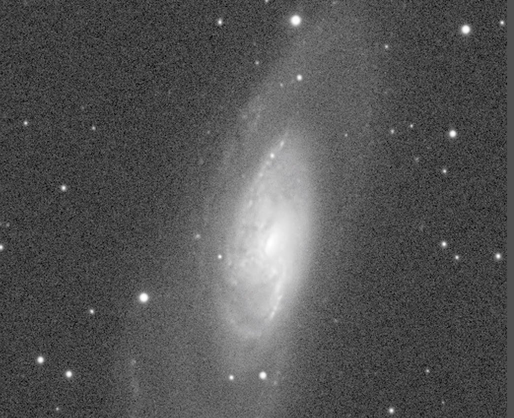
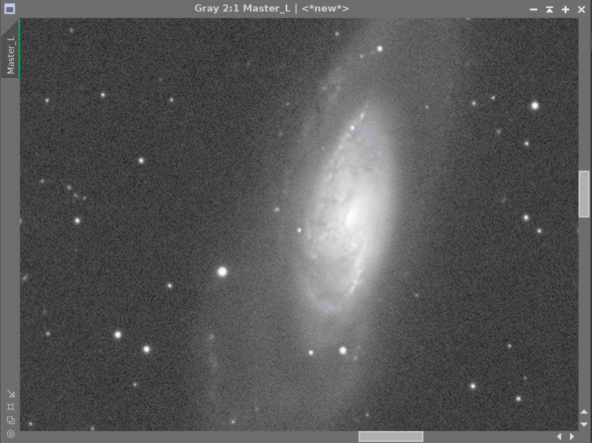
In the next series, I applied LHE to bring out small scale detail. After this I decided to knock down the noise with an Run of Noise XTerminator. When I was done with this, I felt like it would benefit from a LHE run targeting large scale detail and so added the LHE #2 run in. You can see the sequence below in the zoomed in version of the image centered on M106.
Ideally, I should have done both LHE run back to back - but that’s not what I ended up doing…
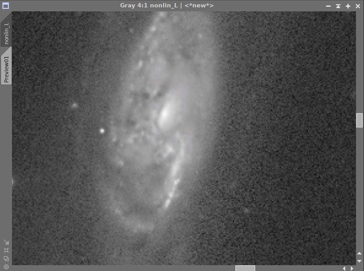
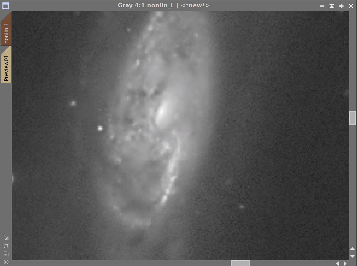
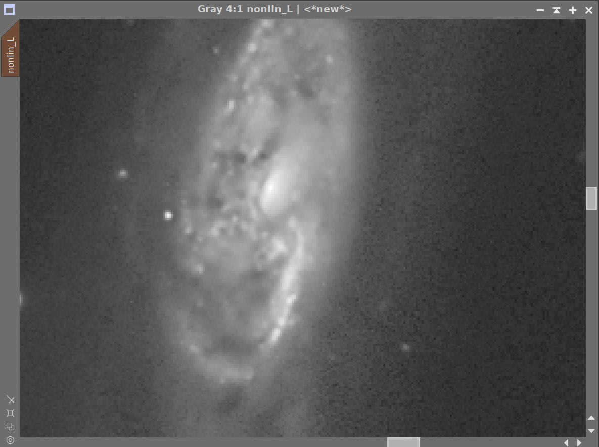
LHE #1, Noise XTerminator (0.6), and LHE #2
11. Create the Initial LRGB Image
Using LRGBCombination tool, fold the L image into the RGB image, creating the first LRGB image
Apply CT to enhance color sat and tone scale
apply the Galaxy Mask
Run ColorSaturaton and CT to adjust galaxy colors.
Run Noise XTerminator with a value 0.6
Invert the mask
Run CT and HT to clean up sky and stars.

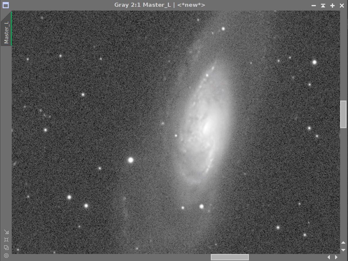
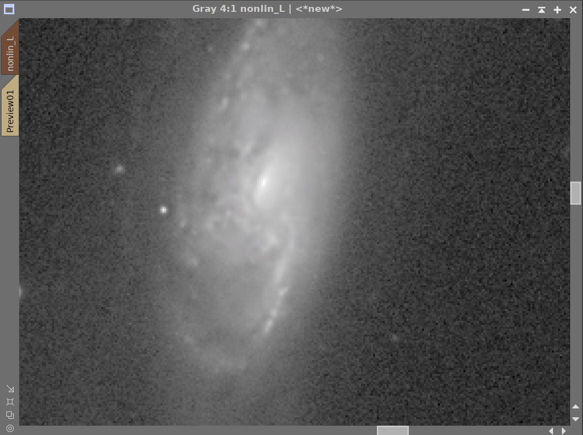
The Nonlinear L imge (on the left) and the Nonlinear RGB image (on the right) before L insertion.

Initial LRGB Nonlinear image after LRGBCombination.
LRGB Image - After CT. (click to enlarge)

ColorSaturation Panel showing color curve applied.

After Applying ColorSaturation and CT on the galaxies alone.

The Galaxy mask has been inverted and HT and CT used to tweak the stars and sky.
12. Reduce Stars
Run EZ-Star Reduction with the Adam Block method.

Before EZ-Star Reduction

After Star Reduction.
13. Export to Photoshop
Save images as Tiff 16-bit unsigned and move to Photoshop
Use Camera Raw Filter to adjust Global Clarity, Texture, and Color Mix
ColorMix is much easier to use to adjust hues in an image compared to the tool provided by Pixinsight and I tend to do this final operation in PhotoShop
Use StarShrink to reduce the largest stars further.
Use lasso with a feather of 25 pixels to select areas around small galaxies
Use camera Raw to enhance the brightness
Use Noise XTerminator to soften edge noise on small galaxies
Add watermarks
Export Clear, Watermarked, and Web-sized Jpegs.
The final image.
The portable scope platform is supposed to be, well, portable. That means light and compact. In determining how to pack this platform for travel, I realized that the finder scope mounting rings made no sense in this application and I changed them out with something both more rigid and compact - the William Optics 50mm base-slide ring set.