
Messier 13 - The Great Hercule Cluster - 8.5 hours in LRGB - Super Sharp!
Date: July 2, 2022
Cosgrove’s Cosmos Catalog ➤#0104

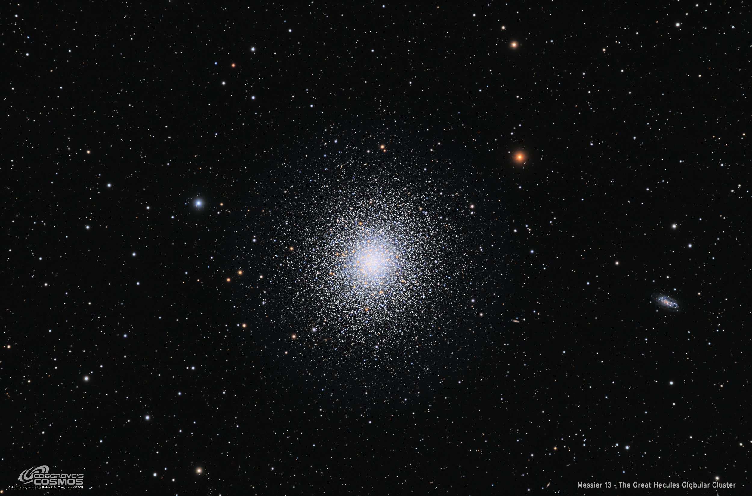
Messier 13 - Taken with the Astro-Physics 130mm APO and the ZWOASI2600MM-Pro camera. Careful culling of unsharp subframes produced some of my sharpest results yet! (Click for the full resolution version via Astrobin.com)
* * This image was published in BBC Sky At Night Magazine - October 2022 issue! **
Thank you much, BBC S@N!

This is a screen snap from my iPhone, as I have a digital subscription!

The image from the Print Issue of the magazine
Table of Contents Show (Click on lines to navigate)
About the Target
Messier 13, also known as NGC 6205, and The Great Hercules Cluster, is broadly regarded as the finest globular cluster in northern skies. It is located 23,150 light-years away in the constellation of Hercules.
M13 is one of about 100 globular clusters that rotate around the center of our galaxy. This cluster consists of anywhere from 100,000 to 500,000 stars packed into a region that is only 135 light-years in diameter. This creates an extremely high density of stars - over 100 times the density found in our local neighborhood. At times stars are so close together that they combine to form new stars that are referred to as “Bue Stranglers”.
This is a very large globular - most globular clusters contain only 10’s of thousand of stars, whereas M13 is an order of magnitude larger. It is also located relatively close to the earth and measures ~ 20’ in diameter - making it large and bright enough to be just be seen with the unaided eye as a fuzzy star.
M13 was discovered by Sir Edmund Halley in 1714 from the island of St. Helena. Charles Messier cataloged it in June of 1764.

Sir Edmund Halley 1656-1742 (image from Wikipedia)

Charles Messier 1730-1817 (image from Wikipedia)
In the image above, a small galaxy, NGC 6702, can be seen about 27’ to the northeast (to the right in the image above). This is a fairly edge-on spiral galaxy that is located 46 million light-years away.

NGC 6207 - a crop from the main image above. 46 Million light-years away!
Another very small edge-on galaxy, IC 4617 is a Seyfert 2 Galaxy and can be seen to the right of the cluster and about halfway between it and NGC 6702. This galaxy is located a whopping 502 million light-years away!
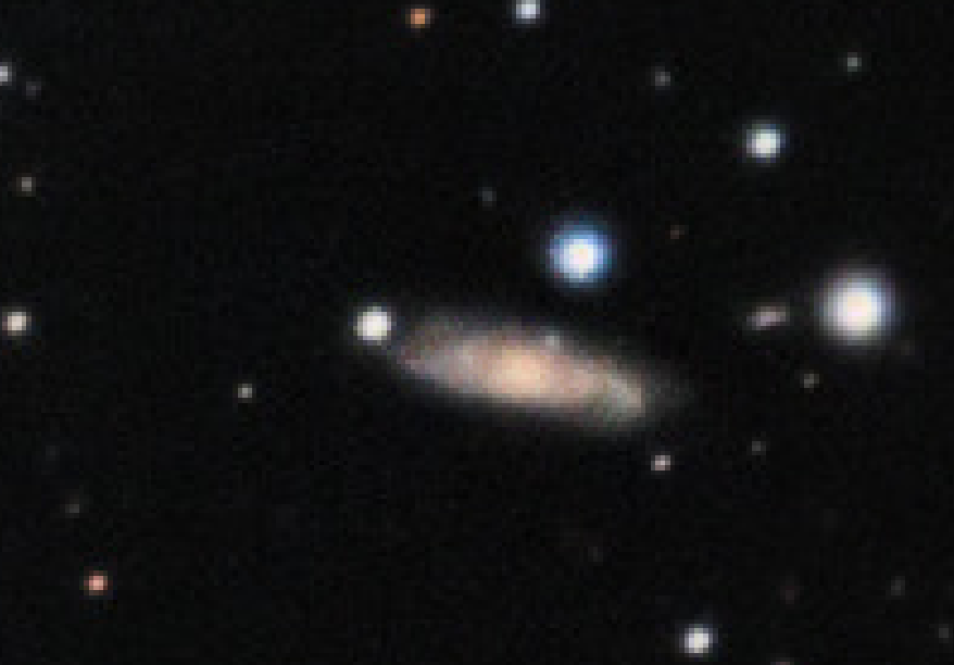
IC 4217 - a crop taken from the image above. 502 Million light-years away!
The Annotated Image
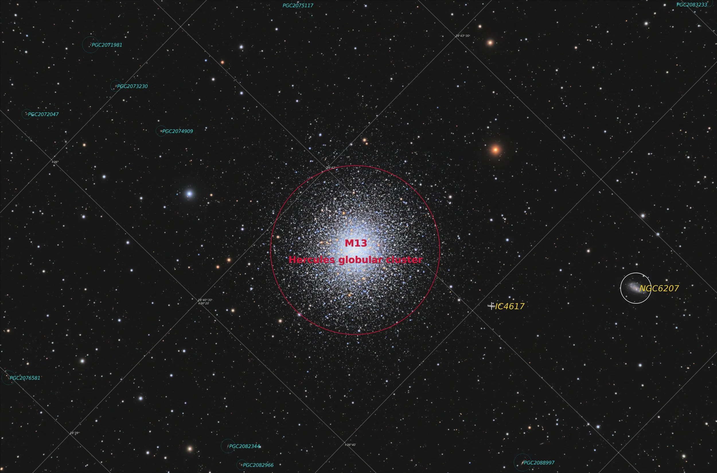
This annotated image was created in Pixinsight, using the ImageSolver and Annotate Image Scripts.
The Location in the Sky

This finger chart was created in Pixinsight using the FinderChart process.
About the Project
Target Selection
We had a great clear stretch of weather from May 29th-31st and I was determined to take advantage of it.
As I reviewed what potential targets would be available, I realized that M13 would be above my treeline by the time we had astronomical darkness. I don’t normally shoot Globular Clusters - but M13 has a special spot in my heart.
Through many years of visual observing, M13 was one of the great targets of summer that was always a treasure to view. No matter what size telescope you had, it was always an impressive view and never a disappointment. I viewed it whenever I had the scope out - and if I had a friend over, it was one of those goto show pieces that I knew would go over well.
I have shot this target before, but I decided to try it again. This time, I wanted to really put my best foot forward.
The first time I shot it was in August of 2019 - in the first weeks after I got my first scope! It was an early test exposure of 10 subs at 60 seconds each - unguided and uncalibrated - because I still did not know how to do those things! In writing this up, I realized that this image was never posted to my website and is, therefore “off the books” - so to speak!
My second effort was done in June of 2020 as a 50-minute integration on my William Optics scope with a ZWO OSC camera.
I shot this a third time on June 3rd of 2021. This was a quick 1.3-hour exposure in LRGB which was shot as a test exposure for my then-new Askar FRA400 portable platform.
This time would be different. I wanted to push for a quality image.
I would use my Astro-Physics 130mm scope - which has my longest focal length of 1080mm. This would provide the best image scale for this object. I would also use my best camera - the ZWO ASI2600MM-Pro camera. I wanted to get as much time as I could over the clear nights there were coming up - I end up getting a total of 8.5 hours. Finally, I would use several new techniques that I had recently mastered to try and get the best quality I could from this image.
Previous Efforts
The Story of the August 2019 shot cannot be seen anywhere as I never added it to my website before - but you can see the image below.
The story of my June 2020 effort can be seen HERE.
The story of my June 2021 effort can be seen HERE.
You can see the comparison of these three shots plus the new one can be seen below:
The June 2019 effort. 10 minutes. No guiding or calibration. Processing in Photoshop.. (click to enlarge)
the June 2021 effort. Test shot for the then new Askar FRA400 with ASI1600MM-Pro camera. (click to enlarge)
The June 2020 effort. William Optics 132mm FLT with OSC camera. (click to enlarge)
The current effort! (click to enlarge)
While the first effort is pretty, shall we say, rough - the other efforts are not half bad. I was pretty proud of each when I did them.
Obviously, the images taken with the William Optics Scope and the OSC camera had good scale and reasonable color. The FRA400 shot has a wider field of view, but the star images are round and crisp and this image validated that the setup using an IOptron CEMM26 mount was capable of great quality output. But the newest one really shines in terms of detail, sharpness, and color.
As an example of that - let’s see what detail I was able to get for the two small galaxies near M13.

NGC 6207 from the current image.

NGC 6207 from the June 2020 effort on the WO 132mm scope

The June 2021 effort on the FRA400 widefield scope

IC 4617 from the current image.

IC 4617 from the June 2020 effort. Note that this galaxy wan not to be seen on the June 2021 effort.
As you can see, the current effort is producing some of the best results I have had to date on this target!
Data Capture
As mentioned before, the images were captured over three nights from May 29th-31st. We have the shortest period of darkness at this time of year, and I got the scope up and running as soon as it was dark enough to start capturing subs.
The nights we clear, calm, and cool. I had no problems at any point in the sequence. I was able to shoot flat cal frames on the first and the third night, and I used the flat frames from the first night to calibrate the second night images.
I knew that sharpness would make or break this image, so I took several steps to help on that front.
I wanted great tracking so I took extra care to very carefully dial-in my Polar Alignment with PoleMaster. Then when I set up PHD2, I took the trouble to run the Guiding Assistant to analyze and optimize guiding parameters.
I always blink images before I begin any processing and one unusual thing with this project was that I found NO problems on any sub taken over these three nights when viewed via Blink! Not one! There were some normal satellite trails and such - but those were of no concern to me. This is the first time in a while that no frames were eliminated due to clouds or other problems.
So the capture session had great clear skies, no Moon, and generated great results!
Image Processing
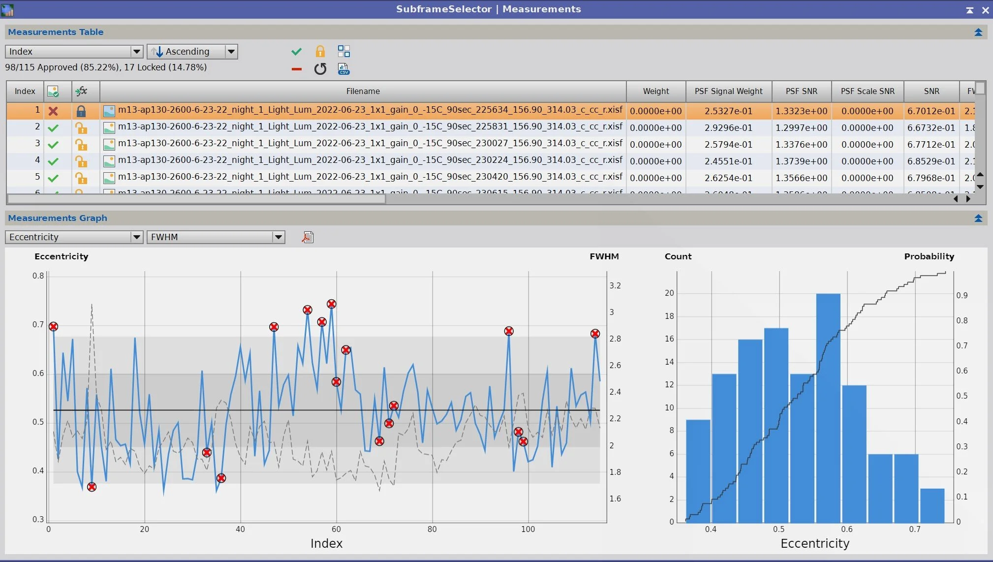
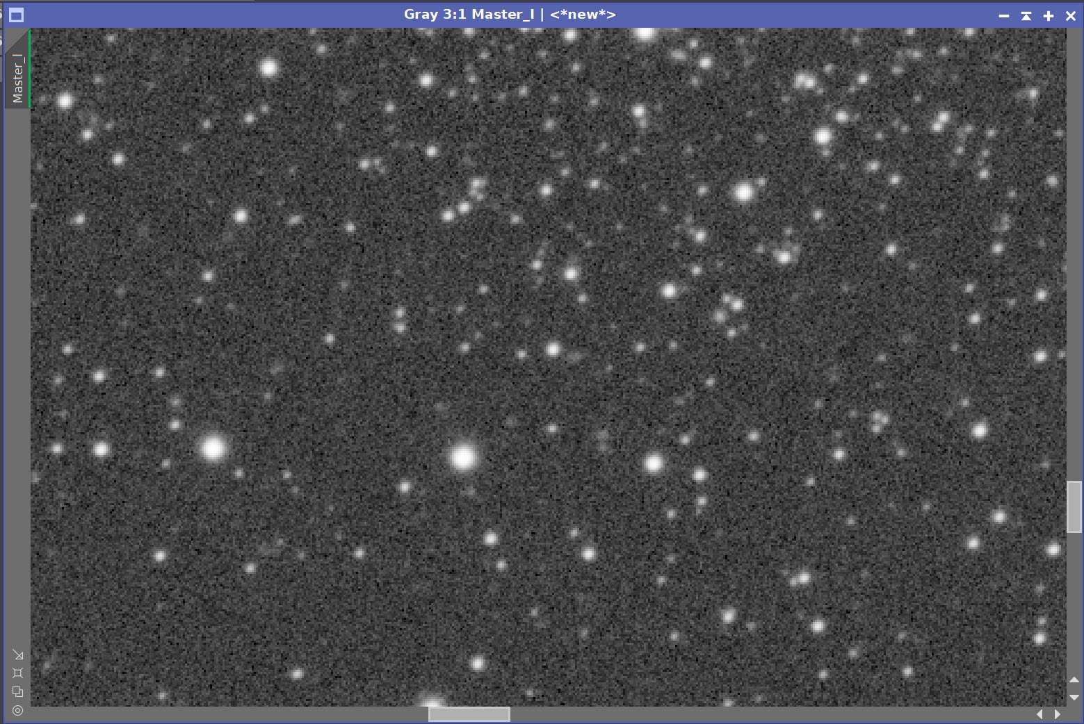
For processing, I followed my typical processing plan, which now includes assessing the calibrated image data with SubFrameSelector prior to image integration. The goal here is to remove subs that will end up potentially hurting the final integrated master. Since sharpness was a key goal here, I was looking for frames that were outliers for FHMN and Eccentricity.
People typically use SubFrameSelector with complex equations that create metrics indicating those frames that should be removed from the set.
My use of SubFrameSelector is much simpler. I am reasonably new to using this tool and what I tend to do is look at the attributes that are key to me achieving my current goal. Lately, I have been on sharpness kick, so the two parameters I just mentioned play into this quite well. A sub with a measure of FHWM that is high relative to the other subs in the set likely has been impacted by passing clouds or a focus issue. Images with guiding issues will tend to have oval stars - and thus higher eccentricity scores.
While it is true that properly set rejection parameters can minimize the impact of such bad frames, sometimes it is best to just pull the sub out of the mix entirely. I try to make sure I have a significant number of subs so that removing the worst one will not have a major impact on my integration times. If my times are already short, I tend not to do this.
The Master images produced in this way were very crisp and showed excellent detail.
Processing Indecision
As I progressed in my processing, I noticed that I was having a difficult time deciding where I wanted to take this image.
I have done a lot of work now processing nebule and galaxies, and I seem to have developed my “inner eye” that allows me to know where I want to take an image. But this did not seem to be the case for this Globular Cluster. I was less confident in my processing decisions.
So I went on Astrobin and did a search for all of the Top Pick Award images of M13 and reviewed them.
As you might imagine, there were as many looks are there were astrophotographers involved, but I did notice one thing. Many of them had diffraction spikes prominently displayed on the bright stars.
Spikes can’t easily be avoided if you have secondary mirror support vanes in your optical tube. Since I don’t get them as I use refractors, I wondered if they added to the aesthetic of the image that I might be missing - perhaps I should add them digitally. So I tried that out:
My Initial Image (click to enlarge)
The same image - this time with phony diffraction spikes. (click to enlarge)
In the past, I always thought these phony diffraction spikes were kind of silly. But I wondered if they helped this kind of image.
So I did what I often do when I am unsure of how to process an image. I shared my early version with a couple of my fellow astrophotographers in the area, Dan Kuchta and Gary Optiz, and asked for their feedback.
The feedback on the spike was clear - dump them! They don’t really look that natural. Since this was my initial assessment as well, that was feedback that was easy to take.
The feedback I received on the image without the garish spikes was mixed. - Gary tended to like it, and Dan thought it did not look as natural as it could:
the background was too dark
the color of the center of the globular was off
the stars were too enhanced and looked a little natural
As I looked at the image again - with this feedback in mind - I did begin to notice things that registered with me once they were called out. Some of the enhanced stars did look a bit unnatural to me. So I created a new version that attempted to address the concerns that Dan had raised.
I thought the new version looked much more natural. I shared this new image with Dan and Gary again. Dan really liked the new version while Gary thought that the first version still had more impact in his opinion.
My Initial Processing(click to enlarge)
My second attempt - with a more natural look (click to enlarge)
So now I had two images with different processing goals and a split decision about which was the better image!
Why would this happen? Because each astrophotographer develops their own inner eye and this drives what they like in an image. Dan and Gary are experienced and accomplished astrophotographers - they know what they like. Neither one is right or wrong. They are in fact both right and I fully respect their opinions.
I then posted both images on Twitter and asked the #Astrophotography community which one they liked best.
So I shot M13 w/Astro-Physics 130mm+ASI2600MM-pro. 8hrs+ in LRGB. culled subs for max sharpness.
— 🔭Cosgrove's Cosmos💫 (@CosgrovesCosmos) July 1, 2022
I processed it 2 ways. 1st is w/ a much darker background & hypersharpened stars. 2nd w/ more natural background & stars.
Which do you prefer?#Astrophotogragraph pic.twitter.com/E0YxExQPlU
I got a lot of responses and each image had its own proponents - but the more natural versions had the most votes.
Here are some samples of the feedback I received:
#2 is more natural and #1 has more ‘optics’ (what you expect to see). Prefer 1 for effect. Great shots both.
— Sriram (@really_sriram) July 2, 2022
Both are magnificent. I’d go with the left, which reveals more stars
— AstroFrontyard (@AstroFrontyard) July 2, 2022
BOY that is a Tough one to pin down for me. They Both are simply Brilliant captures and Processing results.
— The Bloodstone™🎸🔭 (@BS2KZ) July 1, 2022
IF i had to narrow it the Right one for my Tired Eyes.
The first photo. More contrast.👍🏻 Great photo by the way.
— Jay Jay (@bmwfreq) July 1, 2022
Beautiful picture. I prefer the sharper stars of the 1st, but with the more natural sky background of the 2nd.
— Sikke Kingma (@SikkeKingma) July 1, 2022
Wow, these are both just amazing shots. Such incredibly crisp detail! (I do like the one on the right….I am a sucker for natural stars. 😂). But they are both beyond fantastic.
— Tom Bock (@galunga70) July 1, 2022
With all of this input, it was time for me to put my big boy pants on and decide what I liked and make a statement with my final edits.
I have been in this position before. It’s like I have this angel sitting on one shoulder whispering in my ear: “use a light touch - respect nature”. But on my other shoulder, I have this devil shouting in my other ear: “Hit it harder! Make it POP! More Color! More enhancement!” I hate it when they fight - I am left not knowing where I want the image to go!
I could see the pros and cons of each approach. In the end, I decided to blend the two images and see if I liked where they came out.
I tried 25/75, 50/50, and 75/25 blends. For me, the best was the 50-50 blend:

My final image was a 50-50 blend of the the inital more processed image and the second more natural image.
And this is the image that I used as the basis for my final image. I think takes some of the best attributes from each image and avoids some of the pitfalls of each image as well.
A detailed Processing Walk-Through is provided for this image at the end of the posting…
More Information
Wikipedia: Messier 13
Wikipedia": NGC 6207
UniverseGuide.com: IC 4617
EAS NASA Hubble Images: Messier 13
Astronomy Now: Messier 13
Messier-Objects.com: Messier 13
Capture Details
Lights Frames
Data was collected during the Nights of 5-29-22, 5-30-22, and 5-31-22
115 x 90 seconds, bin 1x1 @ -15C, Gain Unity, ZWO Gen II Lum filter
75 x 90 seconds, bin 1x1 @ -15C, Gain Unity, ZWO Gen II Red filter
75 x 90 seconds, bin 1x1 @ -15C, Gain Unity, ZWO Gen II Green filter
75 x 90 seconds, bin 1x1 @ -15C, Gain Unity, ZWO Gen II Blue filter
Total of 8.5 hours
Cal Frames
25 Darks at 120 seconds, bin 1x1, -15C, gain Unity
25 Dark Flats at Flat exposure times, bin 1x1, -15C, gain unity
12 flats Flats at bin 1x1, -15C, gain unity
Software
Capture Software: PHD2 Guider, Sequence Generator Pro controller
Image Processing: Pixinsight, Photoshop - assisted by Coffee, extensive processing indecision and second-guessing, editor regret, and much swearing…..
Capture Hardware:
Scope: Astro-Physics 130mm F/8.35 Starfire APO
built in 2003
Guide Scope: Televue TV76 F/6.3 480mm APO Dublet
Main Fous: Pegasus Astro Focus Cube 2
Guide Fous: Pegasus Astro Focus Cube 2
Mount: IOptron CEM60 - new
Tripod: IOptron Tri-Pier with column extension
Main Camera: ZWO ASI2600MM-Pro
Filter Wheel: ZWO EFW 7x36
Filters: ZWO 36mm Gen II LRGB filters
Astronomiks 36mm 6nm Ha, OIII, & SII filters
Rotator: Pegasus Astro Falcon Camera Rotator
Guide Camera: ZWO ASI290MM-Mini
Power Dist: Pegasus Astro Pocket Powerbox
USB Dist: Startech 7 slot USB 3.0 Hub
Software:
Capture Software: PHD2 Guider, Sequence Generator Pro controller
Image Processing: Pixinsight, Photoshop - assisted by Coffee, extensive processing indecision and second-guessing, editor regret and much swearing…..
Click below to see the Telescope Platform version used for this image
Image Processing Walk-Through
(All Processing done in Pixinsight - with some final touches done in Photoshop)
1. Blink Screening Process
Lum Images: lots of trails, some gradients, none removed!
Red: lots of trails, some gradients, none removed!
Green: lots of trails, some gradients, none removed!
Blue: lots of trails, some gradients, none removed!
Flats: all looks good
Darks: all good
First time in a long time that I did not have to remove any frames due to blink! The data looked really solid!
2. WBPP 2.5
All frames loaded, including darks, flats, and flat darks.
Set up for calibration only - no integration
Cosmetic Correction setup
Use the SELECT button for maximum image quality
Subframe weighting: psf signal
Local Normalization enabled
Grouping Keyword set to "Night"
Cometic correction set to all filters
90 sec Darks mapped for all nights
Missing flats for night 2 mapped to night 1 flats
Linear normalization set for Auto and for the best group of frames
Run completed in 1 hour and 20 minutes with no issues

WBPP Calibration view.

Post Calibration View.
3.0 Use SubFrameSelector to analyze the Calibrated subs
Subs for each filter were loaded into the tool and metrics were computed. FWHM and Eccentricity were the key metrics I used in this analysis. Screenshots for each filter are attached below.
Lum Images: 17 deleted for having either too high an FWHM or Eccentricity value
Red Images: 10 deleted for having too high an FWHM or Eccentricity value
Green Images: 5 deleted for having too high an FWHM or Eccentricity value
Blue Images: 9 deleted for having too high an FWHM or Eccentricity value
I was pretty aggressive on what I eliminated as I had plenty of subs and I wanted the best sharpness I could get.

Lum Sub FWHM - Note eliminated frames

Red Sub FWHM - Note eliminated frames

Green Sub FWHM - Note eliminated frames

Blue Sub FWHM - Note eliminated frames
Lum Sub Eccentricity - Note eliminated frames

Red Sub Eccentricity - Note eliminated frames

Green Sub Eccentricity - Note eliminated frames

Blue Sub Eccentricity - Note eliminated frames
4. Integration
ImageIntegration
ImageIntegration was run for each Master image.
It used the same setup for each run.
RCR was chosen for rejection.
Large scale rejection checked - 2x2
A sample panel for ImageIntegration can be seen below

ImageIntegration panel settings.
Rejection High - Lum: Note trails removed (click to enlarge)

Rejection High - Green: Note trails removed (click to enlarge)
Rejection High - Red: Note trails removed (click to enlarge)

Rejection High - Blue: Note trails removed (click to enlarge)
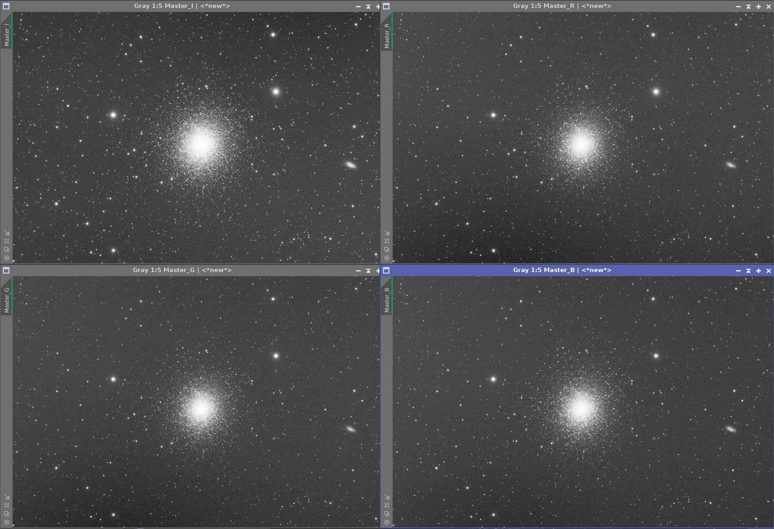
The initial Master images.
5. Crop all of the images
A common crop level was selected and DynamicCrop was used to trim all of the master frames.
6. Dynamic Background Extraction
DBE was run for each image using the subtraction method. Below are the Sampling plans, the before image, the after image, and the removed background images.
DBE: L Sampling (Click to enlarge)
DBE: R Image Sampling (Click to enlarge)
DBE: G Sampling (Click to enlarge)
DBE: B Sampling (Click to enlarge)
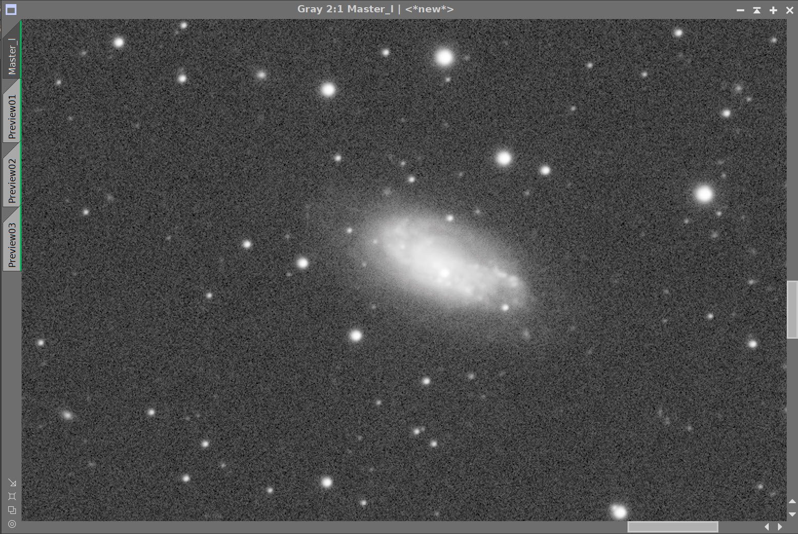
L image Before DBE (click to enlarge)
R Image Before DBE (click to enlarge)
G image Before DBE (click to enlarge)
B image Before DBE (click to enlarge)
L image After DBE (click to enlarge)
R Image After DBE (click to enlarge)
G Image After DBE (click to enlarge)
B image After DBE (click to enlarge)
L background removed (click to enlarge)
R background removed (click to enlarge)
G background removed(click to enlarge)
B background removed (click to enlarge)
7. Create and Process the Linear Color Image
Use ChannelCombination process to create an initial RGB image.
Run DBE on the image to remove any color gradients. Use sampling similar to that used on the mono images, and use subtraction as the correction method,
Run PCC to color calibrate the image
Run Noise XTerminator with a value of 0.5 to “knock the fizz off”
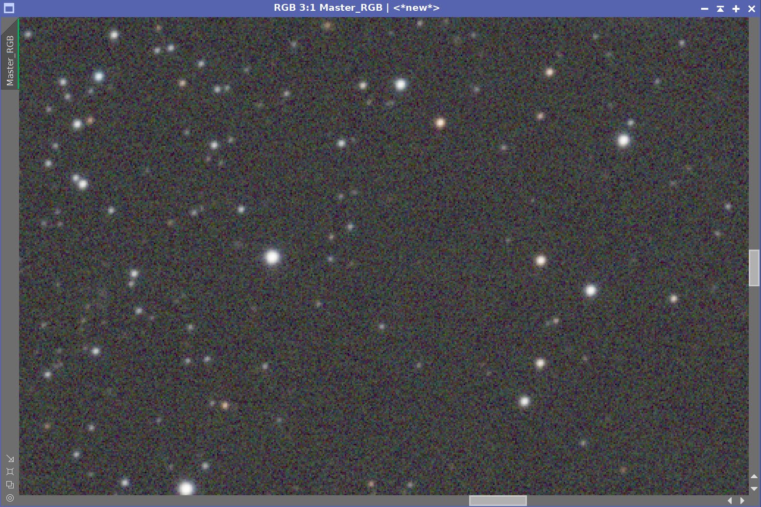
Initial RGB Linear Image (click to enlarge)
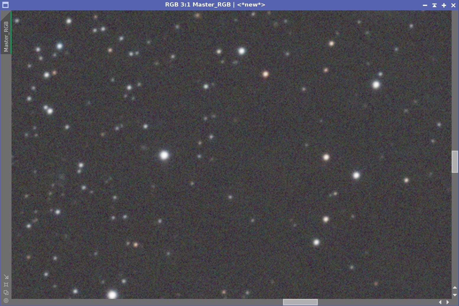
RGB Linear after application of DBE (Click ot enlarge)

PPC was run and the following balance function were computed.
After PCC applied. (click to enlarge)
Before and After application of RC Noise XTerminator with a value of 0.5
8. Take Color Image Nonlinear and Process.
Create a Preview of a good sample of the background sky
Run MaskedStretch on the image - using the sky background preview as a reference.
Use CT to adjust Tonescale and color Sat. Reduce the intensity of the core
Create an M13 mask using the GAME script
Apply mask and do a color sat boost with CT to the cluster.
The image should appear darker and more saturated than desired in preparation for the L image injection.
Initial Nonlinear RGB image after MaskedStretch and CT adjustment. (Click to enlarge)

Mask for M13 created with the GAME Script
After M13 is masked and the saturation boosted with CT (clock to enlarge)
9. Process the Linear L image.
Prep for running Deconvolution
Create a PSF image by running PFSImage Script
Create the Local Deringng Support Image (LDSI)
Create a mask using the StarMask Process - with layers = 6
Adjust with HT to boost stars a bit.
Establish previews on the L image to test deconvolution values.
Test deconvolution parameters iteratively, first determining Global Dark and Global Bright values, then iterations, and finally the Regularization values.
See the values used and results below.
Run Noise XTerminator with a value of 0.5

PSFImage Panel

The final PSF image computed

StarMask Panel with settings used to create the LDSI image.

The Local Deringing Support Image (LDSI)
Decon Preview sample regions used for Deconvolution parameter testing. (click to enlarge)

The deconvolution parameters I ended up using.
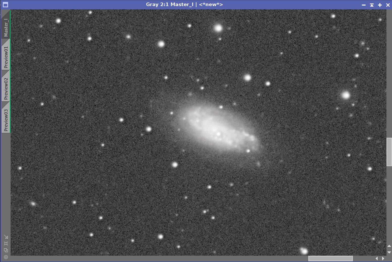
L image: Before and After Deconvolution

L image: Before and After Noise XTerminator with a value fo 0.5
10. Take L image Nonlinear and Process
Take the L image nonlinear
Create a preview that selects a black portion of the sky
Run MaskedStretch using the preview on the liner L image
Using CT, adjust the image
Enhance the smaller features by running LHE run #1:
Kernel radius of 22, contrast limit of 2.0, Amount of 0.5, and an 8-bit histogram
Run CT to final tweak tone scale - making a darker image as the L-insertion will tend to brighten too much or an image like this.
Nonlin L after MaskedStretch (click to enlarge)
Nonlin L after MaskedStretch + CT (click to enlarge)
Nonlin L after the LHE operation. (click to enlarge)
Nonlin L after the final CT adjustment. (click to enlarge)
11. Create the Initial LRGB Image
Using LRGBCombination tool, fold the L image into the RGB image, creating the first LRGB image
Apply CT to enhance color sat and tone scale
apply the Galaxy Mask
Run ColorSaturaton and CT to adjust galaxy colors.
Run Noise XTerminator with a value of 0.6
Invert the mask
Run CT and HT to clean up the sky and stars.
The Nonlinear L image before L insertion. (click to enlarge)
Final RGB image before L insertion (click to enlarge)

Initial LRGB Nonlinear image after LRGBCombination.
LRGB Image - After CT. (click to enlarge)
12. Reduce Stars
Run EZ-Star Reduction with the Adam Block method.


Before EZ-Star Reduction
13. Export to Photoshop
Save images as Tiff 16-bit unsigned and move to Photoshop
Use Camera Raw Filter to adjust Global Clarity, Texture, and Color Mix
ColorMix is much easier to use to adjust hues in an image compared to the tool provided by Pixinsight and I tend to do this final operation in PhotoShop
Use StarShrink to reduce the largest stars further.
Use a lasso with a feather of 25 pixels to select areas around the small galaxies
Use camera Raw to enhance the brightness
Use Noise XTerminator to soften edge noise on small galaxies
Add watermarks
Save several versions of the image as jpegs:
initial image with aggressive enhancements and a darker background for greater contrast and “pop”
a second version with a lighter background, less Clarity, and texture enhancement to the cluster for a more natural look.
An experiment with adding diffraction spikes on the brighter stars.
Share version of the images with colleagues and the Twitter #Astrophotography community and ask for feedback.
Experiment with a blend between the aggressively enhanced versions and the more natural version. A 50-50 blend was chosen as the final version.
Export Clear, Watermarked, and Web-sized jpegs.
The final image.
Adding the next generation ZWO ASI2600MM-Pro camera and ZWO EFW 7x36 II EFW to the platform…