
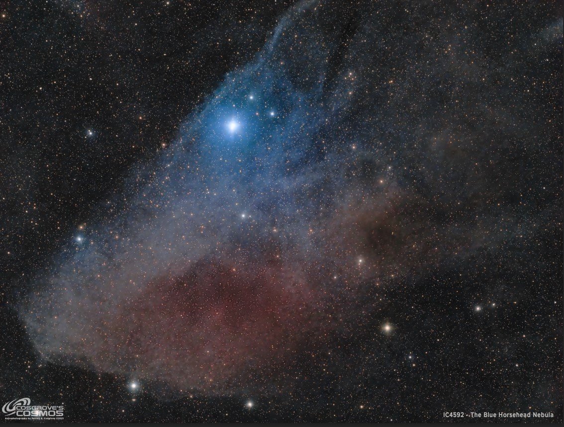
IC 4592 - The Blue Horsehead Nebula - 4.5 hours in LRGB
Date: July 9, 2022
Cosgrove’s Cosmos Catalog ➤#0105

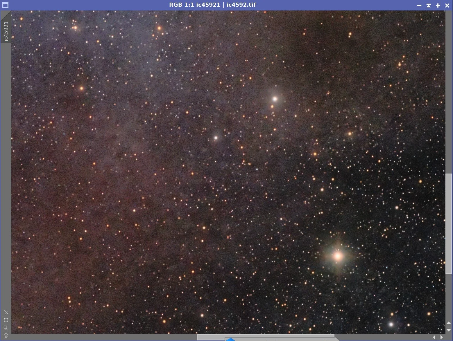
IC 4592 - Taken with the Askar FRA400 Astropraph and the ZWOASI1600MM-Pro camera. (Click for the full-resolution version via Astrobin.com)
Table of Contents Show (Click on lines to navigate)
About the Target
IC 4592, better known as the Blue Horsehead Nebula, is found 400 light-years away towards the center of our Milky Way, in the constellation of Scorpius. This large reflection measures about 3 x 1.5 degrees in size and is part of the Rho Ophiuki Complex.
It gets its blue coloration from the bright star, Nu Scorpii, which forms the "eye” of the horsehead, and illuminates the dust and gas in the nebula.
The Horsehead Nebula is not as well known or photographed as many others. Being large and faint, it is difficult to observe visually and is shown best by deep exposure integrations.
The Annotated Image

This annotated image was created in Pixinsight, using the ImageSolver and Annotate Image Scripts.
The Location in the Sky

This finger chart was created in Pixinsight using the FinderChart process.
About the Project
Target Selection
We are currently still in the tail-end of galaxy season and once again I was struggling to find a target for my 400mm widefield astrograph. After searching around for a while, I noticed that IC 4592 was positioned well for capture.
I should clarify that.
It was positioned as well as it ever will be when seen from MY driveway!
The target is located fairly low in the southern sky and is placed between the narrowest gap in my two tree lines. So - it was as good as I will ever get! With some luck, I could capture about an hour a night of useful exposure for this target.
On top of that, it never gets very high in my skies. It ranged from 22 to 25 degrees above the horizon, so I would be imaging it through a lot of the atmosphere.
Finally - this target is actually pretty large, and even with my 400mm scope, I would have some difficulty fitting it into the field of view.
So - given that this target had several issues - why choose it at all?
Well, for one, I think it is a beautiful target - based on the images I have seen from it.
Plus - all of those challenges? That just makes it all the more interesting to go after!
So I used the Mosaic and Framing Wizard in SGP to carefully compose the image and went off to collect some photons!
Data Capture
The data was captured on the nights of 6-23-22, 6-24-22, 6-25-22, and 7-03-22.
Since my access window was narrow, I made sure that the FRA400 scope was the first one polar aligned and ready to go as soon as I could. The target cleared the trees about 15 minutes after we reached astronomical darkness, and exposures continued until the target hit the other tree line.
In general, tracking was looking pretty good, and I used manual camera rotation on the scope to dial in the precise rotation needed to achieve the specified framing.
I was able to shoot flats each night, so I use a keyword in WBPP to apply the right cal files to the right light images.
For the first three nights, capture seemed to go reasonably well. However, the final night was plagued with thin clouds moving through. PHD2 kept losing the guide stars and SGP’s disaster recovery mode was invoked many times.
Image Processing
I ended up rejecting a lot of subs because of either clouds or trees moving into the field as the target entered the second tree line.
For the most part, the biggest issue I was running into was bloated stars. This was due to two things. First - the low angle of the target meant I was seeing it through a lot of atmosphere - I think this produced worse “seeing” conditions and the brighter stars were allowed to bloat. The other thing that can drive this is the fact that the camera I was using has a reputation for creating haloes and reflections when bright stars are in its field.
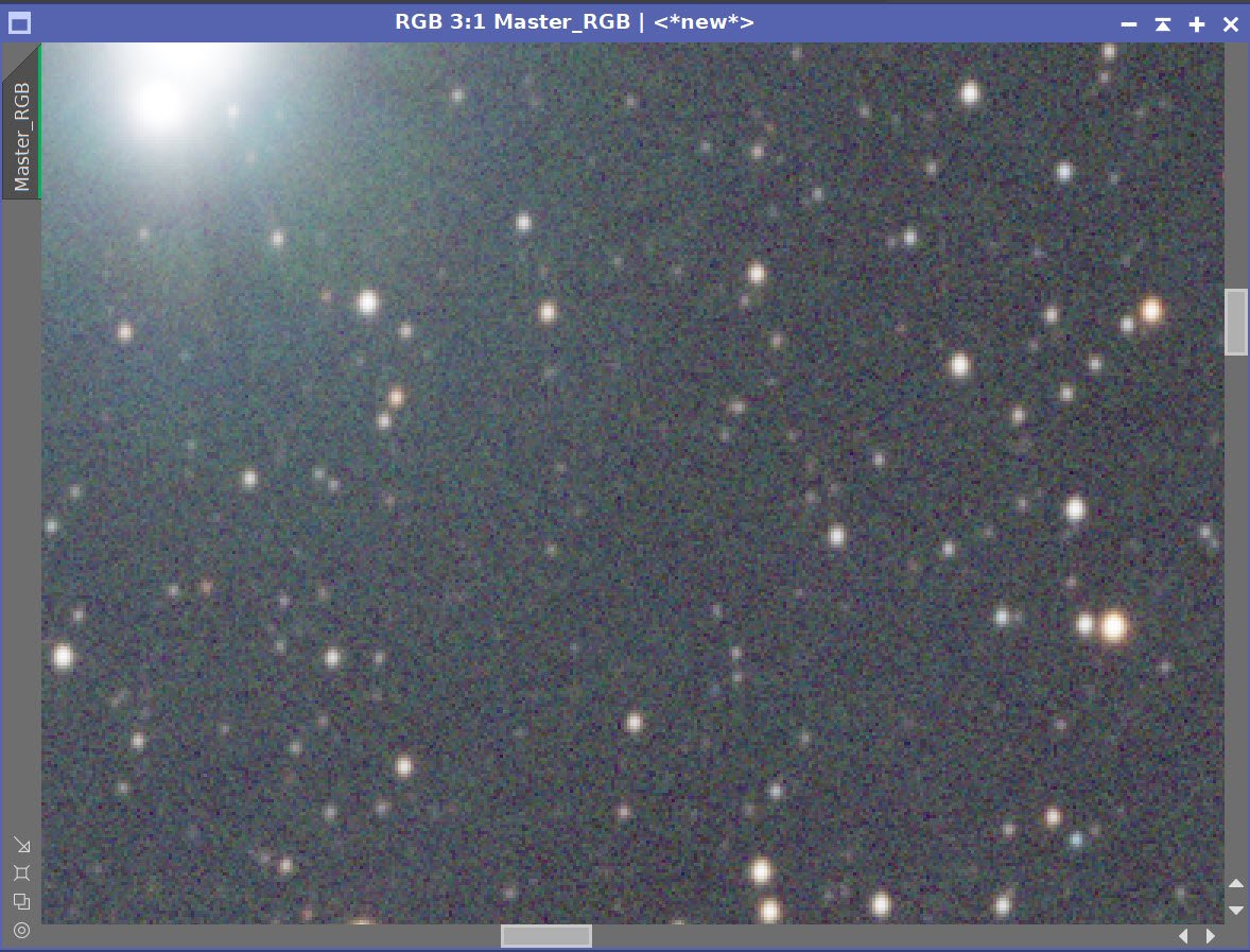
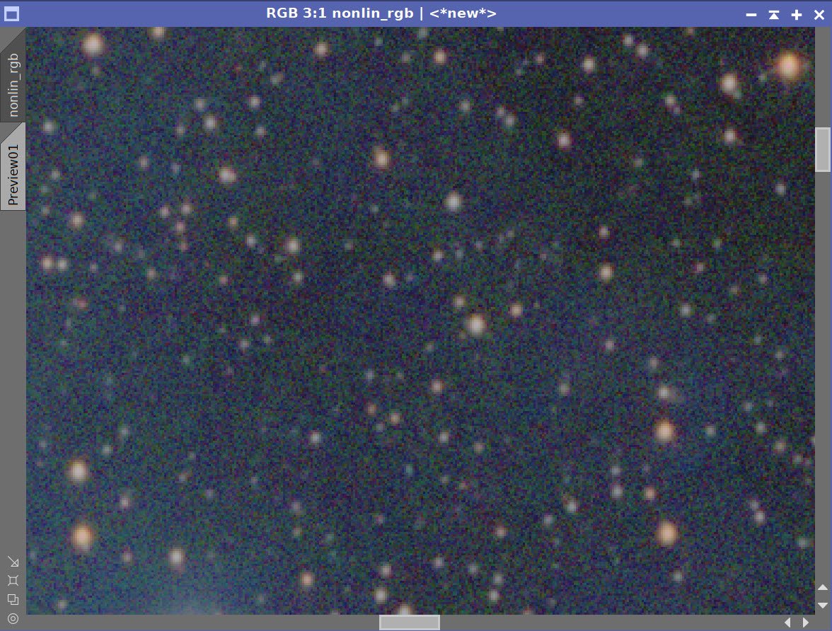
The second problem did not become evident until I was almost done. At that point, I was seeing a pattern in the data that I have seen before - I call this the bubble-pack pattern. This is a medium-scale mottling that seems to occur in areas of the image where noise is high and aggressive noise reduction was applied. I, personally, am very sensitive to this imaging artifact. It can also come about from the use of Local Histogram Equalization tool.
An example of the bubble-pack pattern I am concerned about.
Since the pattern is associated with mid-scale noise, I have often seen this when MLT was used for linear noise reduction. I improved this situation when I started to use EZ-Noise Reduction when working with linear. This script addresses mid-scale noise quite nicely. Recently, I have been using RC Noise XTerminator. I wondered if that might be causing an issue.
I used LHE on the Nonlinear L image - so that was another possible source.
So I went back and reprocessed the image using EZ-Denoise and eliminated the LHE run. The problem was still there.
I think this is just a case where I really needed many more subs to capture the low-intensity nebulosity adequately. With more subs, the noise is reduced and the signal is made cleaner. Of course with my trees and how low the target is to the horizon - I will never likely get more subs on this image - short of trying again next year and adding more subs to the data pool - and I may well do just that.
So - what can I do about it?
I used the ExtractLayers script to pull out 8 layers of detail. I inspected each layer and I found the pattern seemed to be routed in layers 4 & 5. So I tried using MLT with layers 5 and 6 eliminated and this did tend to help.
So I created a mask with GAME to isolate the areas that exhibited the problem the most and then applied MLT to mute the problem. This seemed to work, but I was not really happy with the final result.

MLT reduction of layers 4 and 5 helped a bit. But I really just need more subs!
I think the final answer for me will happen once I can get more subs - perhaps next year.
For now, I think this result will have to stand as it is.
A detailed Processing Walk-Through is provided for this image at the end of the posting…
Capture Details
Lights Frames
Data was collected during the Nights of 6-29-22, 6-30-22, 6-31-22, and 7-03-22
37 x 120 seconds, bin 1x1 @ -15C, Gain Unity, ZWO Gen II Lum filter
31 x 120 seconds, bin 1x1 @ -15C, Gain Unity, ZWO Gen II Red filter
33x 120 seconds, bin 1x1 @ -15C, Gain Unity, ZWO Gen II Green filter
36 x 120 seconds, bin 1x1 @ -15C, Gain Unity, ZWO Gen II Blue filter
Total of 4.5 hours
Cal Frames
25 Darks at 120 seconds, bin 1x1, -15C, gain Unity
25 Dark Flats at Flat exposure times, bin 1x1, -15C, gain unity
12 flats Flats at bin 1x1, -15C, gain unity, taken on each evening
Software
Capture Software: PHD2 Guider, Sequence Generator Pro controller
Image Processing: Pixinsight, Photoshop - assisted by Coffee, extensive processing indecision and second-guessing, editor regret, and much swearing…..
Capture Hardware:
Scope: Askar FRA400 f/5. 6 Astrograph
Focus Motor: ZWO EAF 5V
Guide Scope: William Optics 50mm guide scope
Guide Scope Rings: Wiliam Optics 50mm Clamping Ring Set
Mount: IOptron CEM 26
Tripod: Ioptron 1.5” Tripod
Camera: ZWO ASI1600MM-Pro
Filter Wheel: ZWO EFW 1.2 5x8
Filters: ZWO 1.25” LRGB Gen II, Astronomiks 6mm Ha, OIII,SII
Guide Camera: ZWO ASI290MM-Mini
Dew Strips: Dew-Not Heater strips for Main and Guide Scopes
Power Dist: Pegasus Astro Powerbox Advanced
USB Dist: Pegasus Astro Powerbox Advanced
Polar Alignment Cam: Iplolar
Software:
Capture Software: PHD2 Guider, Sequence Generator Pro controller
Image Processing: Pixinsight, Photoshop - assisted by Coffee, extensive processing indecision and second-guessing, editor regret, and much swearing…..
Click below to see the Telescope Platform version used for this image
Image Processing Walk-Through
(All Processing done in Pixinsight - with some final touches done in Photoshop)
1. Blink Screening Process
Lum Images:
Some trails - not many
5 subs were removed because of trees
1 removed for clouds
Some gradients
Red:
Some trails
Some gradients
Removed 3 subs for trees
Removed 3 subs for clouds
lots of trails, some gradients, none removed for that!
Green:
Removed 3 subs for trees
Removed 6 subs for clouds - mostly from the last night
lots of trails, some gradients, none removed!
Blue:
Lots of small trails
Some gradients
1 sub removed for trees
Flats: all looks good
Darks: all good
Flats: All look good, Collected nights 1,2,3 and 4
2. WBPP 2.5
Reset Files
Select Max Quality Preset.
ADD night keyword
Select output directory
Add all files
Enable CC for all files
All frames loaded, including darks, flats, and flat darks.
Set up for calibration only - no integration
Ran and saw that there was an error when local normalization was applied - I have never had this problem before. I therefore decided to apply NSG manually after the fact. See details before.

WBPP Calibration view.

Post Calibration View.
3.0 ImageIntegration
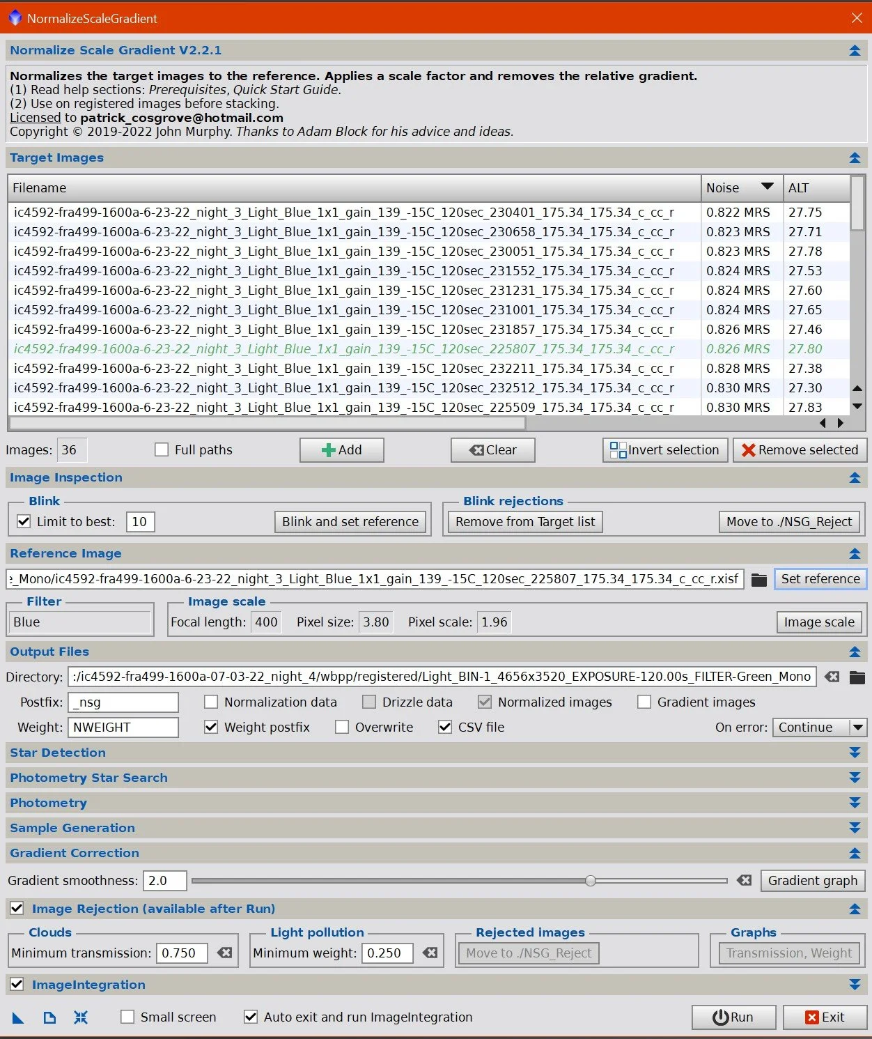
Since Local normalization failed in WBPP, decide to run the NormalizedScaleGradient script. This will normalize each frame to the gradient of the reference frame, and then run ImageIntegration to get to a master file.
I chose the highest altitude image to be the reference image in each case.
Default parameters were used for the most part, however, I did add: Large scale rejection checked - 2x2 for ImageIntegration.
See panel snaps below.

NSG Panel Settings for Lum images.

NSG Red Panel

NSG Green Panel
NGC Bue Panel
NSG Lum Gradient plot (click to enlarge)
NSG Red Gradient plot (click to enlarge)
NSG Red Gradient plot (click to enlarge)
NSG Red Gradient plot (click to enlarge)

ImageIntegration Panel for Lum

ImageIntegration Panel for Green

Rejection High Map: Lum

Rejection High Map: Green

ImageIntegration Panel for Lum

ImageIntegration Panel for Blue
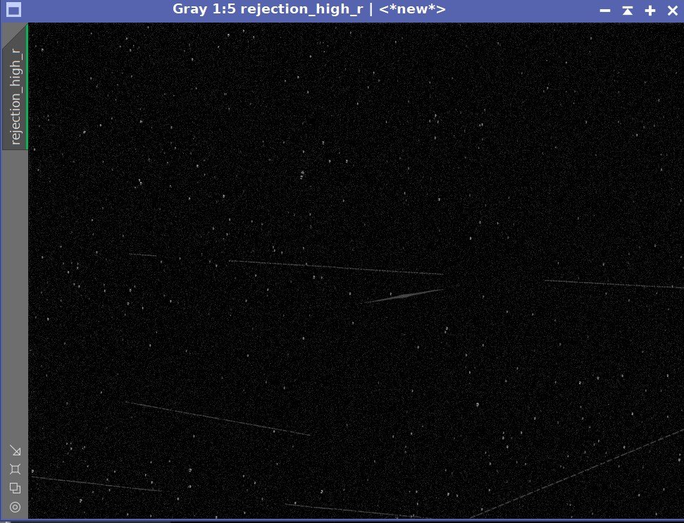
Rejection High Map: Red

Rejection High Map: Blue

The initial Master images - after crop and DBE.
4. Crop all of the images
A common crop level was selected and DynamicCrop was used to trim all of the master frames.
5. Dynamic Background Extraction
DBE was run for each image using the subtraction method. Below are the Sampling plans, the before image, the after image, and the removed background images.
DBE: L Sampling (Click to enlarge)
DBE: R Image Sampling (Click to enlarge)
DBE: G Sampling (Click to enlarge)
DBE: B Sampling (Click to enlarge)
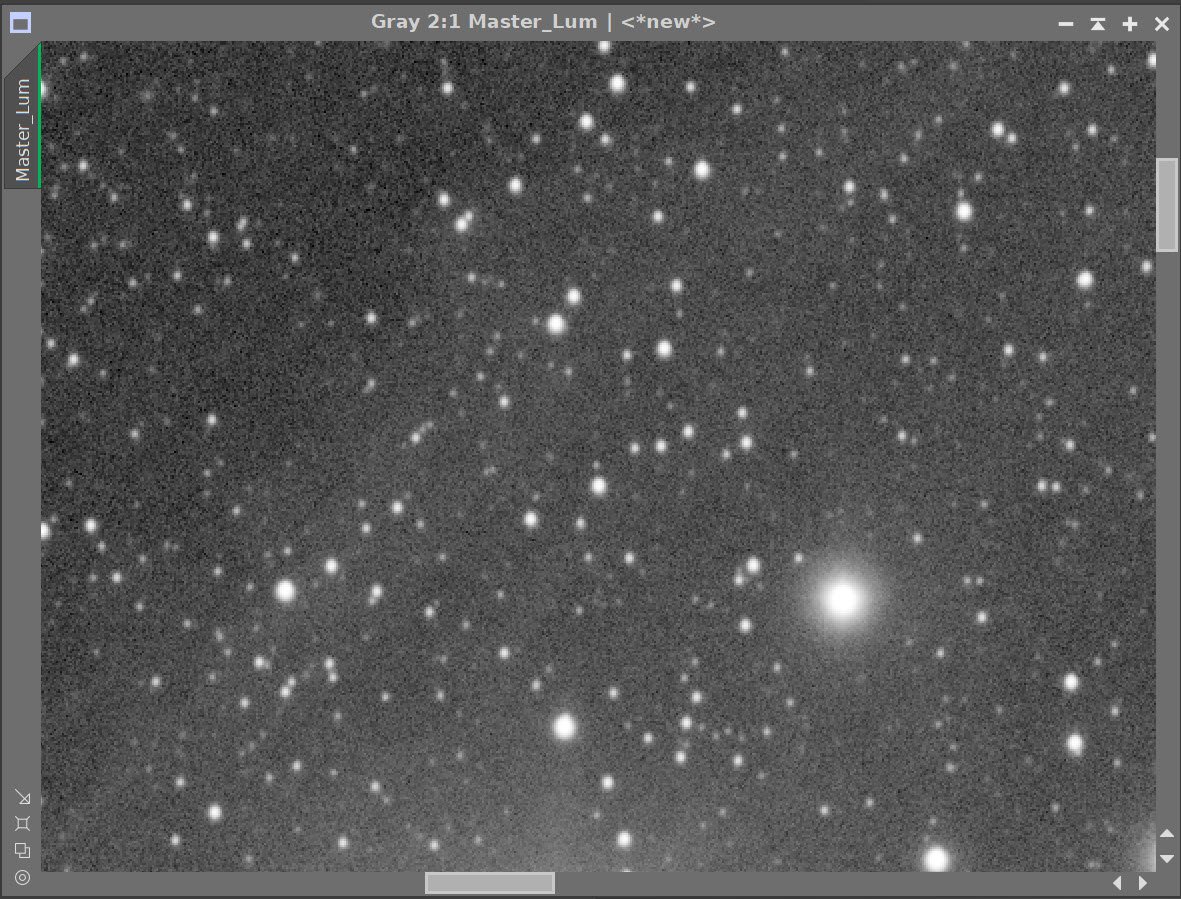
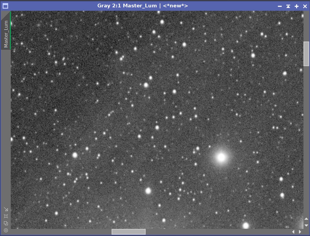
L image Before DBE (click to enlarge)
R Image Before DBE (click to enlarge)
G image Before DBE (click to enlarge)
B image Before DBE (click to enlarge)
L image After DBE (click to enlarge)
R Image After DBE (click to enlarge)
G Image After DBE (click to enlarge)
B image After DBE (click to enlarge)
L background removed (click to enlarge)
R background removed (click to enlarge)
G background removed(click to enlarge)
B background removed (click to enlarge)
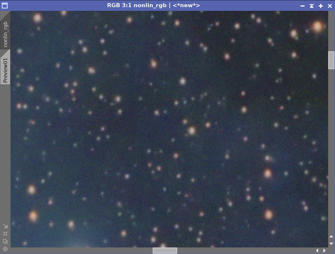
6. Create and Process the Linear Color Image
Use ChannelCombination process to create an initial RGB image.
Run DBE on the image to remove any color gradients. Use sampling similar to that used on the mono images, and use subtraction as the correction method,
Run PCC to color calibrate the image
Run Noise XTerminator with a value of 0.6 to “knock the fizz off”
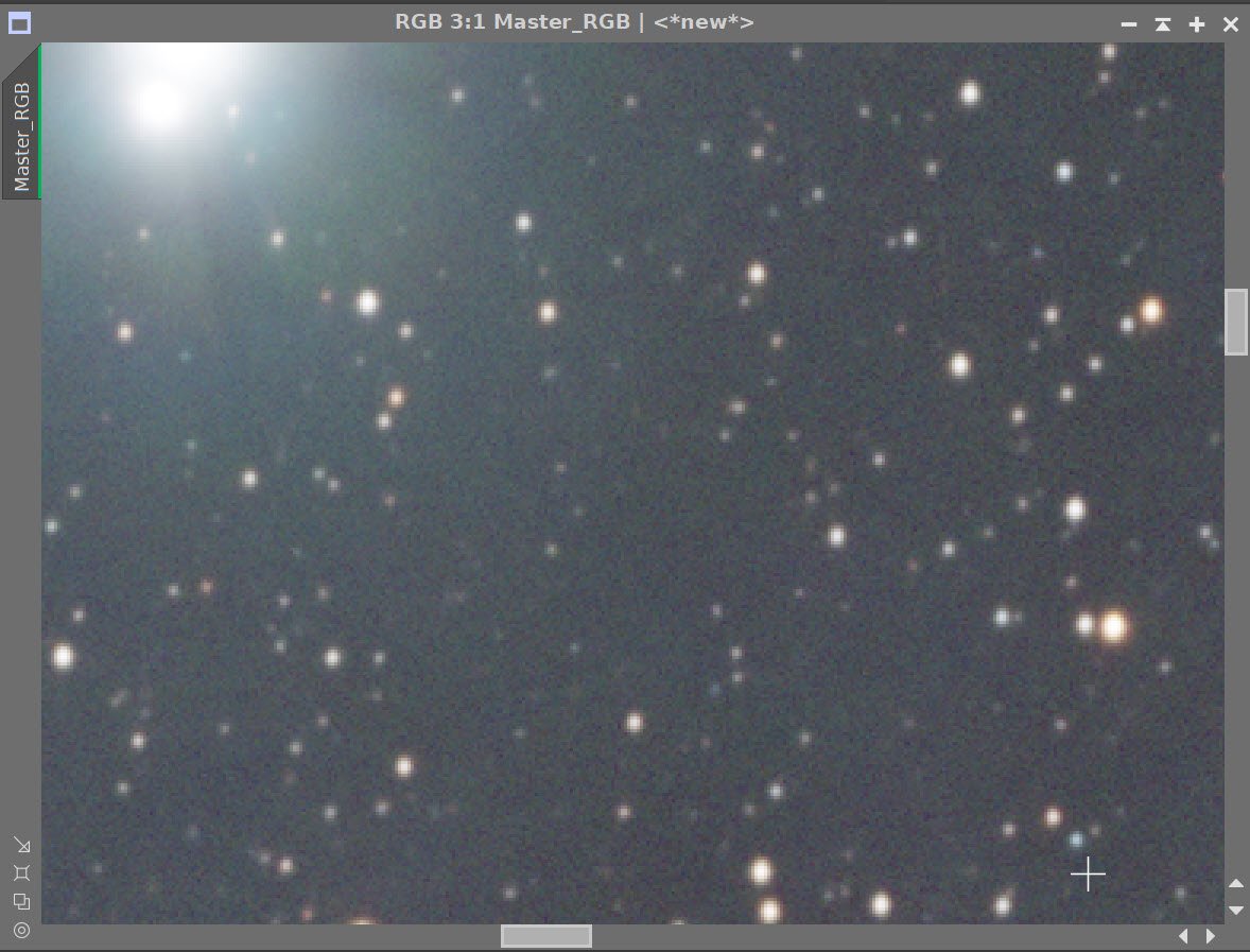
Initial RGB Linear Image (click to enlarge)
RGB Linear after application of DBE (Click ot enlarge)

PPC was run and the following balance function were computed.
After PCC applied. (click to enlarge)
Before and After application of RC Noise XTerminator with a value of 0.6
7. Process the Linear L Image
Prep for running Deconvolution
Create a PSF image by running PFSImage Script
The camera/scope combination undersamples a bit and as a result, the final SF is a bit on the “blocky” side. Normally I would have drizzle processed this image to improve on this, but this image - by its nature- does not have a lot of sharp detail so I did not do that here. I expect Deconvolution to have a relatively minor effect here.
Note - I will not be using an object mask for this effort. Instead, I will be using the Deregularization parameters to protect decon from noise.
Create the Local Deringng Support Image (LDSI)
Create a mask using the StarMask Process - with layers = 7 (there are some larger stars in this image so I increased the layers by one)
Adjust with HT to boost stars a bit.
Establish previews on the L image to test deconvolution values.
Test deconvolution parameters iteratively, first determining Global Dark and Global Bright values, then iterations, and finally the Regularization values.
See the values used and results below.
Run Noise XTerminator with a value of 0.5

PFSImage Panel showing the computed PFS model.

The PFS Image used. Note that it appears a bit “blocky”.

Starmask Panel settings used to produce the LDSI mask.

Here is the HT curve I used to boost the stars size of the LDSI mask.
The final LDSI image used. (click to enlarge)
These preview areas were used to test various Deconvolution parameter values. (click to enlarge)

These were the final values for decon determined by testing.
Before and After Deconvolution is applied on the L Master Image
8. Take Color Image Nonlinear and Process.
Create a Preview of a good sample of the background sky
Run MaskedStretch on the image - using the sky background preview as a reference.
Use CT to adjust Tonescale and color Sat. Reduce the intensity of the core
Run DBE to remove any residual color gradients
Do a final CT tweak: The image should appear darker and more saturated than desired in preparation for the L image injection.
Apply Noise XTermnator with a value 0.7.
Initial Nonlinear RGB image after MaskedStretch (Click to enlarge)
After an additional tone scale and saturation boost with CT (click to enlarge)
Nonlin RGB DBE Sampling. (click to enlarge)
Before DBE Applied. (click to enlarge)
After DBE Applied. (click to enlarge)
Background removed (click to enlarge)
Before and After RC Noise XTerminator (0.7)
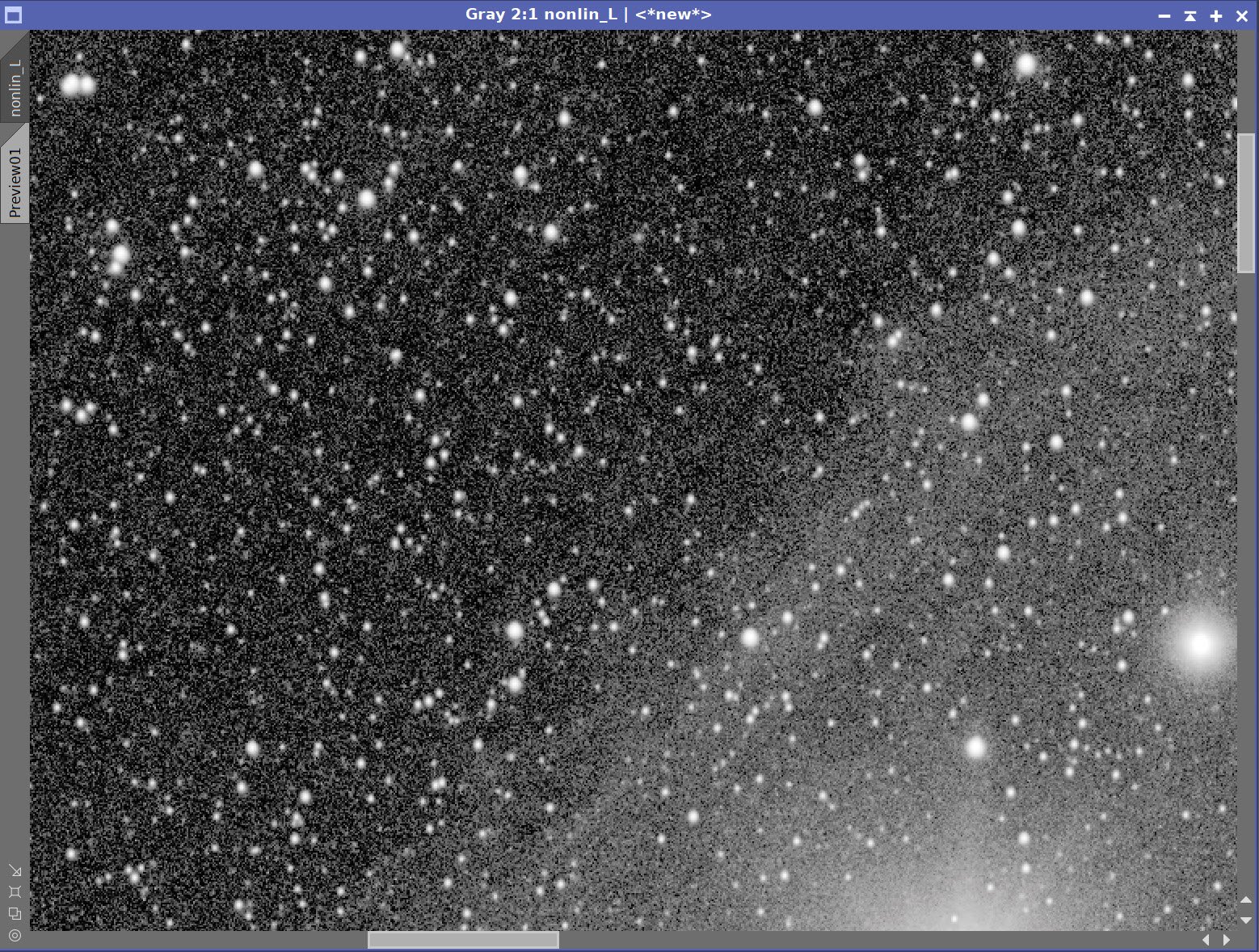
9. Take L image Nonlinear and Process
Take the L image nonlinear
Create a preview that selects a black portion of the sky
Run MaskedStretch using the preview on the liner L image
Using CT, adjust the image
Enhance the larger features by running LHE 360, 2.0,0.2, 12-bit
Run RC Noise XTerminator with a value of 0.7
Nonlin L after MaskedStretch (click to enlarge)
Nonlin L after CT and LHE applied (click to enlarge)

Before and After RC Noise XTerminator (0.6)
10. Create the Initial LRGB Image
Using LRGBCombination tool, fold the L image into the RGB image, creating the first LRGB image
Apply CT to enhance color sat and tone scale
Run ColorSaturation to tweak color
Run Noise XTerminator with a value of 0.5

Final L and RGB image prior to LRGBCombination.
Initial LRGB Nonlinear image after LRGBCombination. (click to enlarge)

Color Saturation adjustments made.
LRGB Image - After CT. (click to enlarge)
After Color Saturation changes. (click to enlarge)
11. Reduce Stars
Run EZ-Star Reduction with the Adam Block method.

Before Star Reduction

Before EZ-Star Reduction
12. Bubble Pack Problem
A “bubble pack” pattern was seen in the red area(mostly)
Tried alternative processing to use EZ-Denoise rather than Noise XTerinator in linear images. Typically bubble-pack pattern is a mid-scale noise reduction artifact. No difference was seen!
Tried Removing LHE process from nonlinear L image. Bubble-pack patterns can be generated by LHE. No difference was seen. The scale of LHE used was much greater than the bubble pack problem anyways.
I concluded that this was just due to not having enough integration on faint areas.
I range ExtractWavelets for 8 layers. I found that the pattern was rooted in layers 4 and 5.
I created a mask for the red area that showed the problem the most and applied it.
I then ran MLT eliminating these two layers. This seemed to help a bit.
An example of this bubble pack pattern.

Extracted Wavelet Layer #4 - showing part of the pattern

Extracted Wavelet layer #5 - also showing the problem.

After MLT: The pattern is muted but not eliminated. I guess I just need more subs here!
13. Export to Photoshop
Save images as Tiff 16-bit unsigned and move to Photoshop
Use Camera Raw Filter to adjust Global Clarity, Texture, and Color Mix
ColorMix is much easier to use to adjust hues in an image compared to the tool provided by Pixinsight and I tend to do this final operation in PhotoShop
Use StarShrink to reduce the largest stars further.
Use a lasso with a feather of 25 pixels to select areas around the large stars
Use camera Raw to adjust curves and color around these stars to take them a bit.
Do another run of Noise XTerminator in PS to polish the image.
Add watermarks
Export Clear, Watermarked, and Web-sized jpegs.
The final image.
The portable scope platform is supposed to be, well, portable. That means light and compact. In determining how to pack this platform for travel, I realized that the finder scope mounting rings made no sense in this application and I changed them out with something both more rigid and compact - the William Optics 50mm base-slide ring set.