
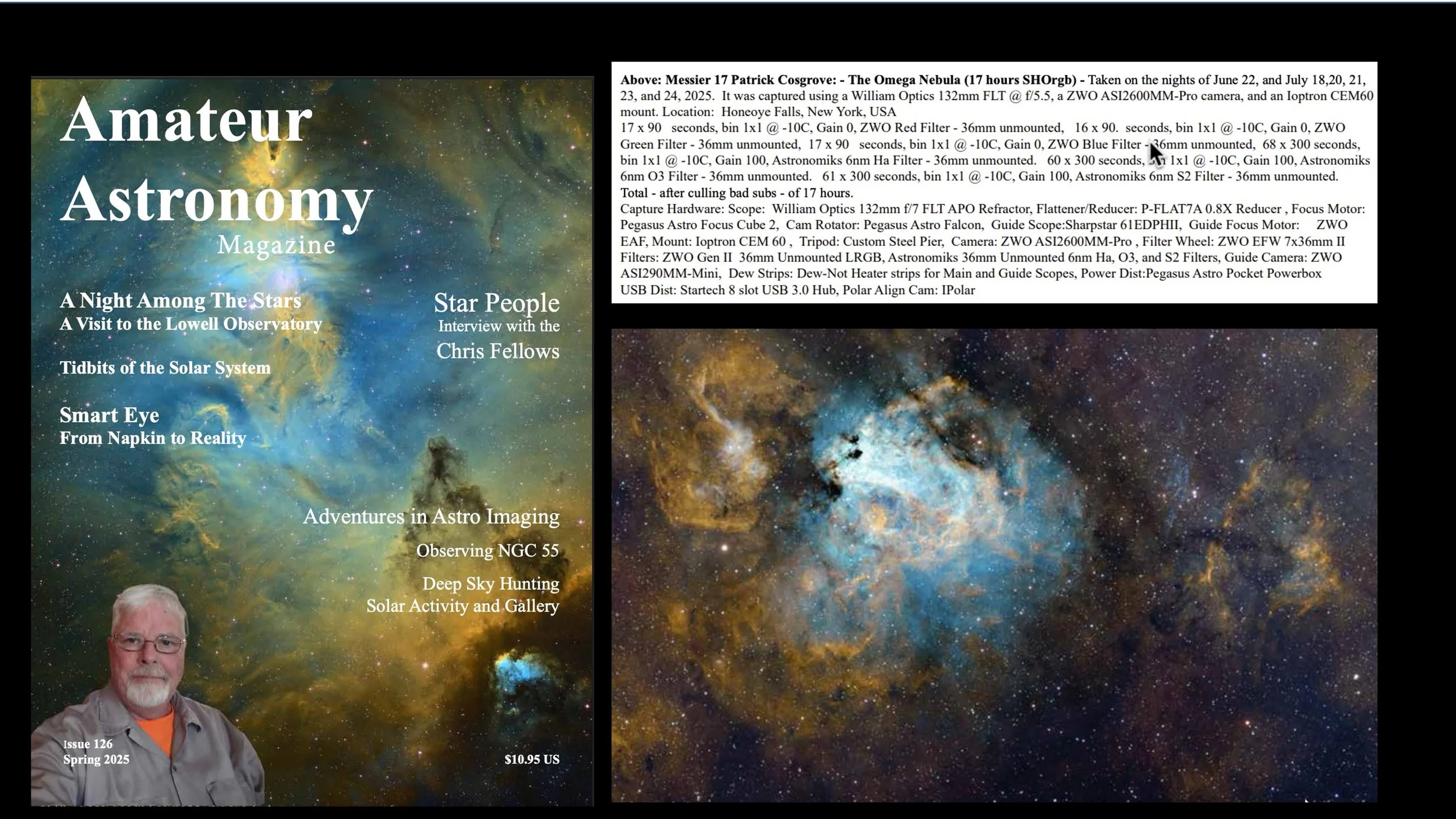
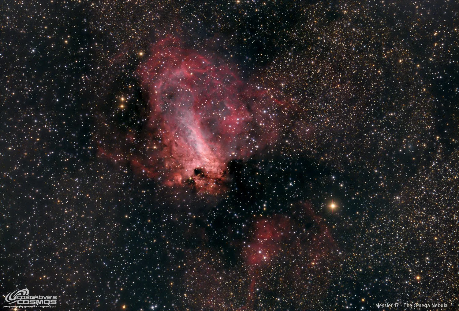
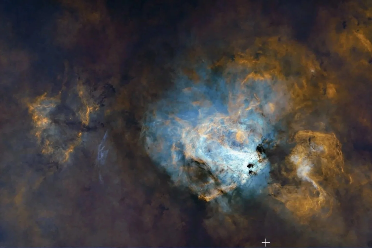
Messier 17 - The Omega Nebula - Victory After Heartbreak! (17 hours SHOrgb on M17!)
Date: July 29, 2025
Cosgrove’s Cosmos Catalog ➤#0143

After losing two complete nights of data, I was finally able to collect 17 hours of integration to create thi simage (click on the image for a high res view via Astrobin.com)
Published in Amateur Astronomy Magazine, Fall 2025, Issue #128
Award “Explore” Status on Flickr!

Table of Contents Show (Click on lines to navigate)
Victory After Heartbreak
The nights are very short now.
Imagine that you have collected three nights of data before the weather window closed.
You pull in all of the data, anticipating a fun image processing session.
You blink the images - and to your horror, all of the images from nights 2 and 3 are out of focus and unusable!
AHHHHHHHHHHHHHHHarg…..
Two clear nights - completely wasted!
I was sick at heart.
M17 was now very low in the sky, and it would be hard for me to collect more data.
But collect, I did.
A few hours every night, I could. Slowly, I built my integration back up.
The story of how this happened and how I recovered is detailed below.
But first, let’s talk about this target and this image…
About the Target
Messier 17 is a bright HII region in the summer Milky Way. While most often known as the Omega Nebula, you will also find it listed as the Swan, Horseshoe, Lobster, Check-mark (and, yes, even the rather indelicate “Tobacco-Pipe”) Nebula, faithful catalogue numbers M 17 and NGC 6618 in tow.
It nestles in northern Sagittarius, a couple of degrees above the “Teapot’s” spout, some 5,500 light-years from Earth—give or take a few hundred, depending on which study you read.
Physically, M 17 is a vast cloud of hydrogen gas lit up by the ultraviolet glow of the embedded open cluster NGC 6618. In visible light, the brighter gas forms a swan-shaped arc about 15 light-years long, but infrared and radio observations reveal a much larger molecular complex—roughly 40 light-years across—hiding enough raw material to build tens of thousands of suns. The cluster already hosts at least nine O-type stars and hundreds of early B-type cousins, whose combined stellar winds carve out cavities and trigger successive waves of star-birth along the nebula’s “neck.”
This sea of ionised gas is exactly why narrowband imaging shines here. This Hubble-palette exposure isolates sulphur-, hydrogen-, and oxygen-emission lines, mapping them to RGB and letting the sculpted shock fronts pop in golds and teals, while adding unfiltered RGB stars keeps the stellar colours honest. In other words, science and aesthetics shake hands—always a pleasant outcome in astrophotography.

Jean-Philippe Loys de Cheseaux 1718-1751 (credit: Wikipedia
Swiss astronomer Jean-Philippe Loys de Chéseaux first recorded the nebula in 1745, describing it as “the tail of a comet.” Charles Messier independently spotted and catalogued it on 3 June 1764 during his famous hunt for non-cometary fuzzballs. Later observers—keen on creative naming—likened its luminous bar to the Greek letter Ω, a graceful swan, or a galloping horse’s shoe, ensuring the object would never suffer an identity crisis again.
Curious tidbits: in the 1950s, distance estimates to stars in M 17 (and its neighbours, M 8 and M 16) provided some of the first solid evidence that the Milky Way possesses spiral arms—the workhorse Sagittarius Arm passes right through this region. Modern infrared surveys (Spitzer, SOFIA, VISTA) keep raising the stellar head-count, uncovering deeply embedded protostars and revealing turbulent bow shocks—smiley-shaped arcs racing through the gas at supersonic speeds. Meanwhile, radio observations show polycyclic aromatic hydrocarbons (the same complex molecules found in barbecue smoke—please resist the urge to inhale) glowing along the nebula’s dusty edges.
Annotated Image
Created in Pixinsight using the ImageSolver and AnnotateImage scripts.
The Location in the Sky
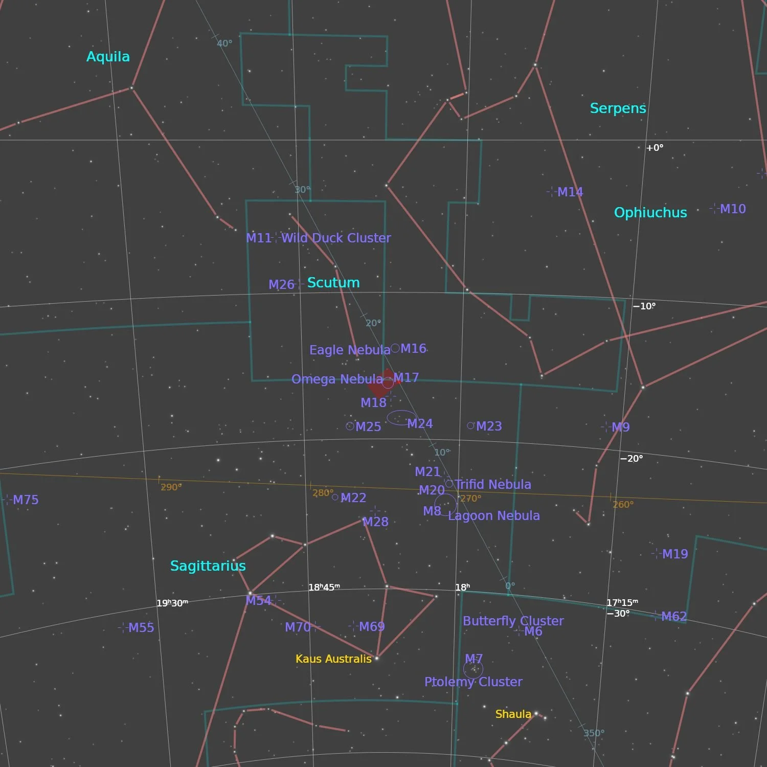
This annotated image created with Imagesolver and FInderChart Scripts in Pixinsight.
About the Project
This is the second imaging project from my Williams Optics 132mm (WO132) Platform, taken from my new Whispering Skies Observatory!
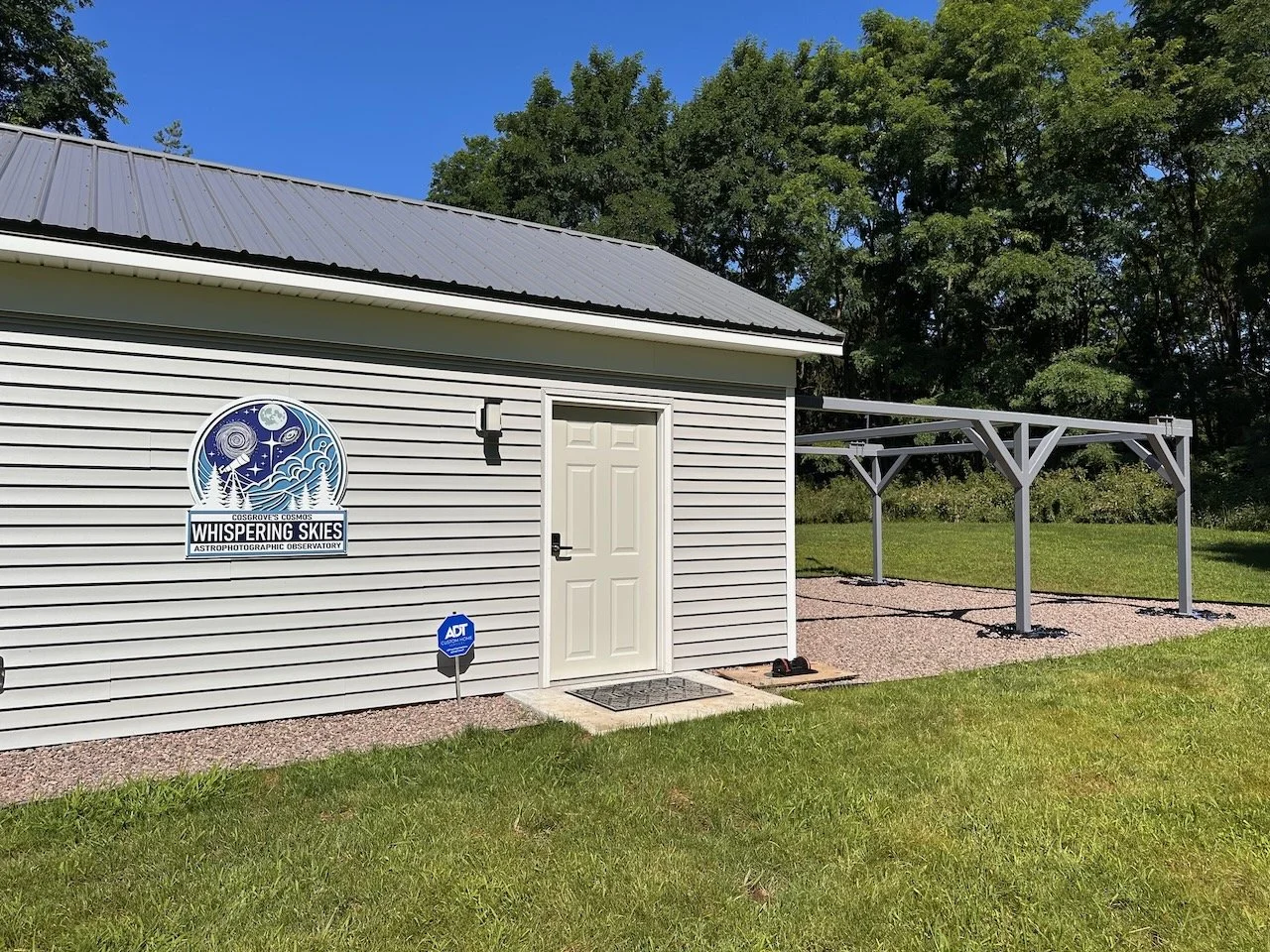
Whispering Skies vatory - outside view.
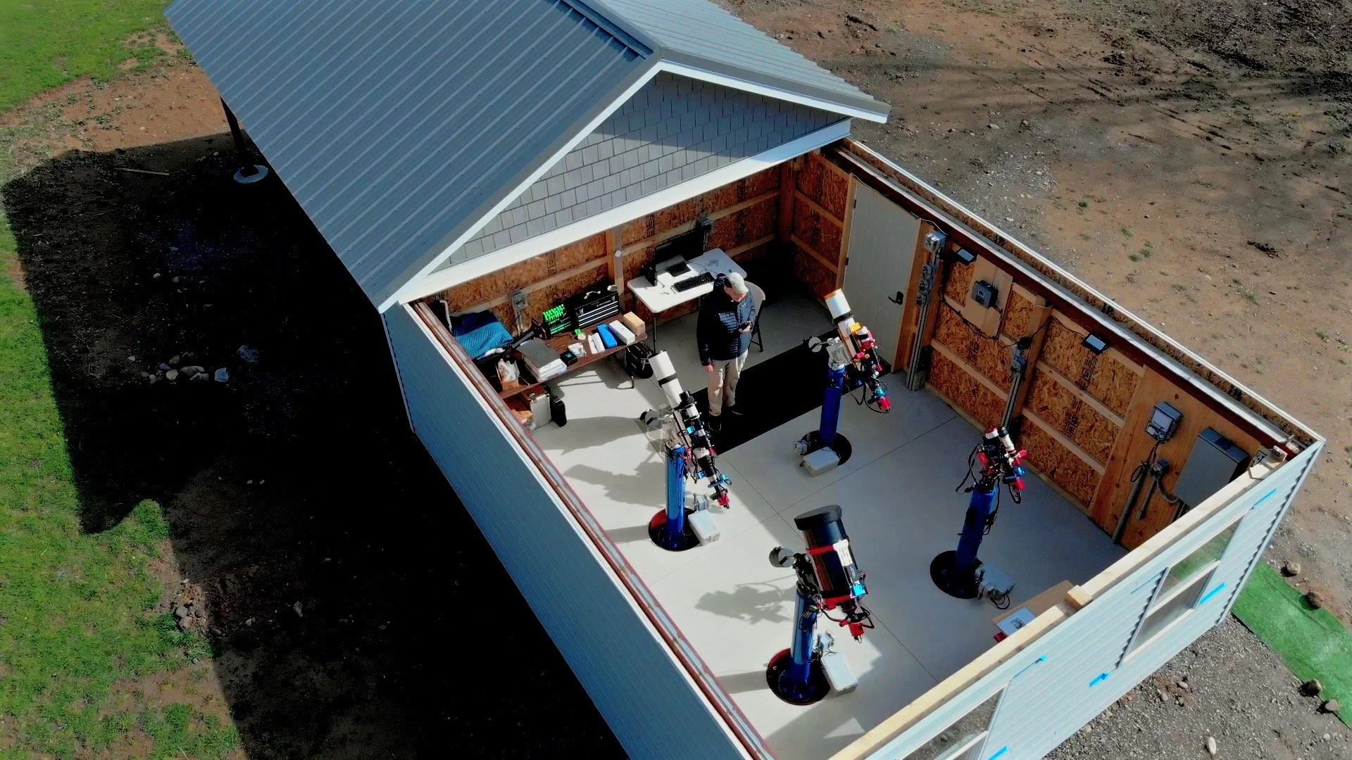
Drone view showing the 4 telescope platforms.
Picking the Target
In the third week of June, we were anticipating some clear skies, and I sat down to draft a target list for my four telescopes.
One of the steps I take as part of this process is to review target lists from previous years. I look for targets that were on my list that I never got to.
As I did this, I came across M17. I remember thinking that this would be a cool object to shoot in narrowband.
I had done this target once before. You can see that here:
M First Attempt at M17 back in 2020. (Click to lmage to go to that post)
This was the result of 1.6 hours using an OSC camera. This was taken in my first year of astro imaging, and I was always kind of proud of this image.
Not long after this was taken, I switched to a mono camera, which allowed me to use either LRGB or Narrowband configurations.
It was clear that this target was an active HII region that should look great in narrowband.
In June, this target was well-positioned, and I planned on shooting it with my William Optics 132mm platform. With the reducer/flattener in place, this system has a focal length of 720mm and runs at a fast f/5.5.
I framed the target such that some of the other faint nebulosity in the region could also be seen.
Data Collection
Starting late on June 22nd, I shot all night then and again on the next clear nights on the 23rd and the 27th.
These were very hot days and nights, and due to this, I set the camera cooler's target temperatures to -10 °C. I knew there was no way they were going to achieve my normal aim of -15 °C.
Everything looked good - or so I thought.
Tracking was good, and the images I saw on the NINA control screen promised a wealth of gaseous detail to explore once data collection was complete.
After the 27th, the weather window closed, and I shot my cal frames the very next night.
The next day, I was eager to process this image.
So I blinked everything, as I normally do.
And as soon as I did this, I was agast to see a large number of images that were out of focus enough to make them useless. In the end, NONE of the subs collected on the second and third nights were useful. It was a crushing disappointment!
Disaster
What happened?
I am set up in NINA to use Focus Offsets.
Before a sequence starts, the system performs autofocus using the Luminance filter. Then it uses a table of focus motor step offsets needed to maintain focus for each filter relative to the luminance focus point.
This means I can put in the Ha filter and take a sub, rotate to the O3 filter and grab a sub, and then the S2 filter - one right after the other. This way, I always have a balanced number of subs for each filter.
In the past, I would autofocus on the filter to be used, shoot a series of X subs, and then change the filter and rerun autofocus before continuing. This much autofocus wastes time that could be used in a sub-collection. It also means that if I get shut down, I may end up with a misbalanced set of subs from each filter.
With the new method, if the weather shuts me down - as it typically does - I have a balanced number of subs allowing me to process what I have.
This new method is significantly more productive. After each sub, the routine examines the star sizes and, if they are growing beyond a specified point, the system pauses the sub collection and reruns autofocus.
It’s always worked well for me - until now.
My initial theory of what went wrong involved the heat. It’s been extremely hot, and I thought this could have altered the dimensions of the scope, rendering the focus offset table outdated.
Rerunning the focus offset routine appeared to resolve the issue.
However, after digging deeper, I now believe I selected the incorrect profile for NINA for these nights, which utilized an outdated focus offset table.
So you know - operator error. Stupid Operator. Sometimes I don’t know how I put up with him… err, me.
So now what?
I did not have enough data to proceed. Getting more was problematic. I wasn't sure if a weather window would open up. But I did know that this target is getting low in the sky, and each night my window to shoot this target would shrink.
So - is this project a bust?
The Observatory to the Rescue!
The whole point of having an observatory is convenience. No long setup times. No long take-down times.
I decided to keep the M17 sequence ready to go in NINA.
As it is now, if we have a good night, I do the following:
Open the observatory after dinner and let it cool down
At near dusk, I go to the observatory, power up the scopes, get all the devices connected in NINA, and fire it off
NINA waits until a few minutes before dark and sets things up, then waits for the target to clear the horizon
Subs run until Dawn or I shut them down
Then I put the dustcaps on the scope and close the roof
Sleep.
During July, we had a string of very iffy nights. But I fired things up - just in case.
The nights always started out looking nice, but at some point or another, clouds came in and put a damper on things. But by taking advantage of these partial nights, I slowly built up more time on target.
When I imported everything into Pixinsight, I was surprised to see that I had a total of 17 hours of integration time. 17 hours on M17!
For me, this was very unusual - the partial nights I would not have gotten without the observatory are really paying off for me now!
Processing Overview
This was a bright nebula target, and as such, I did not feel it needed drizzle processing. So the processing done was pretty straightforward and followed my standard workflow for a SHOrgb image - which can be seen below.
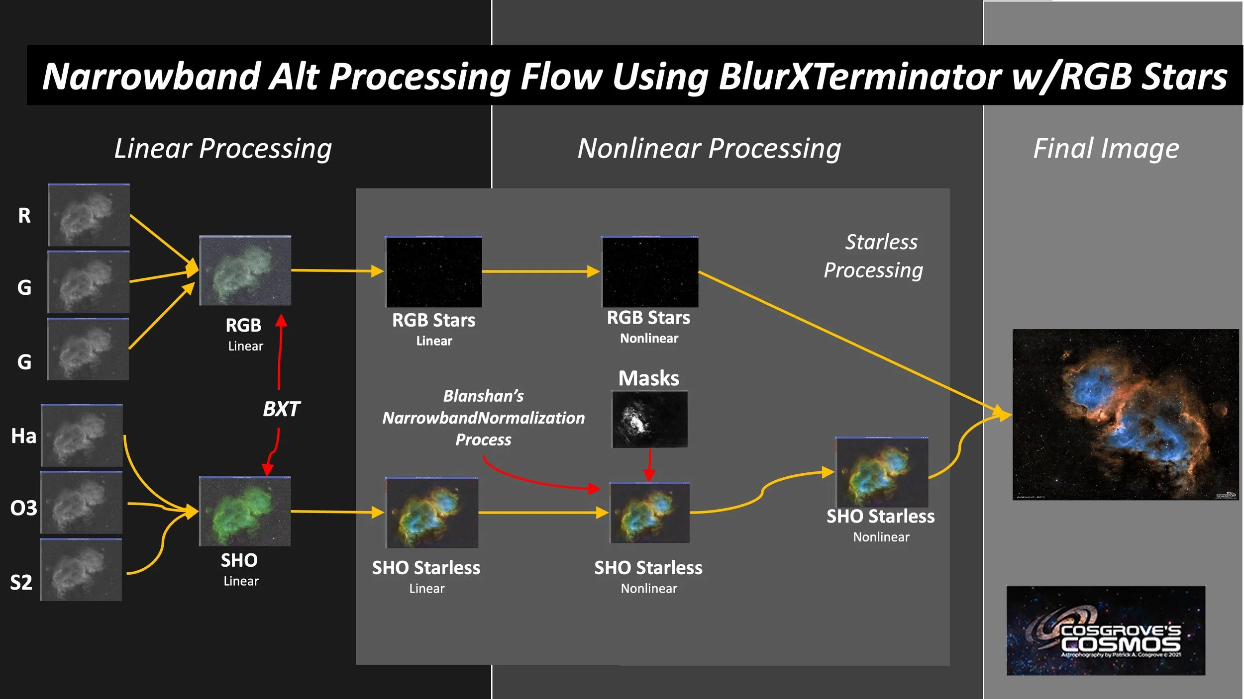
My typical SHOrgb Starless Workflow.
With this image, I have continued to experiment with some of the free scripts available. I want to experience these tools firsthand and see if I like the way they work.
When taking the RGB stars and the SHO Starless images nonlinear, I used Seti Astro’s Star Stretch and Statistical Stretch tools. These worked well for me on this project. I have not really relied on Seti Astro’s tools that much because I have found the user interfaces to be a bit awkward to use, but these did just fine.
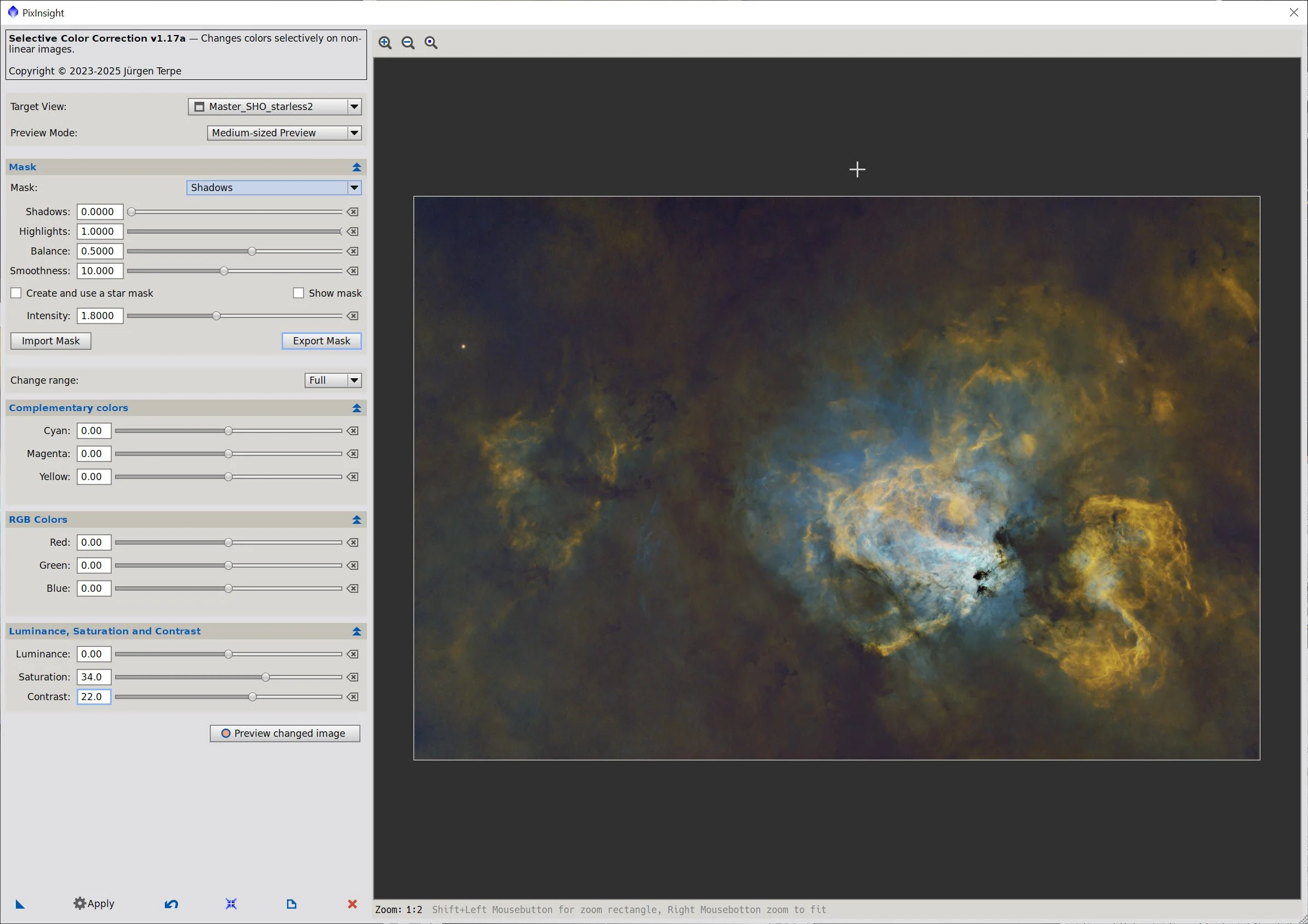
I also used the SelectiveColorCorrection Script to perform most, but not all, of my masked color operations. This script is part of the PixInsight Toolbox created by Jürgen Terpe. This approach worked well and yielded some positive results.
I normally apply LocalHistogramEqualization or MLT sharpening, sometimes targeting specific color regions. But when I tried that for this image, I often found that the look was overprocessed. The 17 hours on target and the nature of the target seemed not to need this, so you won’t see any of that applied here.
Look below for the complete step-by-step walkthrough of the processing. Note: This walkthrough is based on Pixinsight.
Final Results
I am really happy with where this image came out. Lots of detail and color with a look that does not look overprocessed to my eye.
What do you think?
More Information
🖼 High-Resolution Image Galleries
ESA/Hubble – “A Perfect Storm of Turbulent Gases” — Iconic close-up revealing sculpted gas pillars; full-resolution TIFFs available.
NOIRLab Gemini Near-IR Swan — FLAMINGOS-2 infrared mosaic that peers through dust into the hidden stellar hatchery.
Spitzer – “Celestial Sea of Stars” — Mid-IR panorama highlighting warm dust and embedded protostars.
APOD – Star Factory Messier 17 (2024-08-29) — Wide-field composite with narrowband data for colour-palette inspiration.
🔬 Research & Data
The Young Stellar Population in M 17 Revealed by Chandra — 2006 X-ray census of 886 sources mapping NGC 6618’s youthful stars.
The Extended Environment of M 17: A Star-Formation History — 2009 study tracing sequential star-birth across the surrounding molecular cloud.
Spitzer – “Flying Dragon” (M 17 SWex) — Popular-science look at the furious protostar nursery just southwest of the bright nebula.
🔭 Observer’s Corner
Sky & Telescope – M 17: The Nebula with Too Many Names — Visual-observer notes, sketches, and filter tips for backyard telescopes.
🕰️ Fun & Historical Perspective
NOIRLab – Mayall 4-m Photo (1973) — Vintage film image showing M 17’s grandeur before the CCD era.
NASA – “A Perfect Storm of Turbulent Gases” Press Release — Explainer likening the nebula’s internal weather to a cosmic hurricane—plywood not required.
Capture Details
Lights Frames
Taken the nights of June 22, and July 18,20, 21, 23, and 24, 2025
17 x 90 seconds, bin 1x1 @ -10C, Gain 0, ZWO Red Filter - 36mm unmounted
16 x 90 seconds, bin 1x1 @ -10C, Gain 0, ZWO Green Filter - 36mm unmounted
17 x 90 seconds, bin 1x1 @ -10C, Gain 0, ZWO Blue Filter - 36mm unmounted
68 x 300 seconds, bin 1x1 @ -10C, Gain 100, Astronomiks 6nm Ha Filter - 36mm unmounted.
60 x 300 seconds, bin 1x1 @ -10C, Gain 100, Astronomiks 6nm O3 Filter - 36mm unmounted.
61 x 300 seconds, bin 1x1 @ -10C, Gain 100, Astronomiks 6nm S2 Filter - 36mm unmounted.
Total - after culling bad subs - of 17 hours.
Cal Frames
25 Darks at 90 seconds, bin 1x1, -10C, gain 0
25 Darks at 300 seconds, bin 1x1, -10C, gain 100
30 Dark Flats at Flat exposure times, bin 1x1, -10C, gain 0 for RGB and gain 100 for narrowband
One set of Flats done:
15 R Flats
15 G Flats
15 B Flats
15 Ha Flats
15 O3 Flats
15 S2 Flats
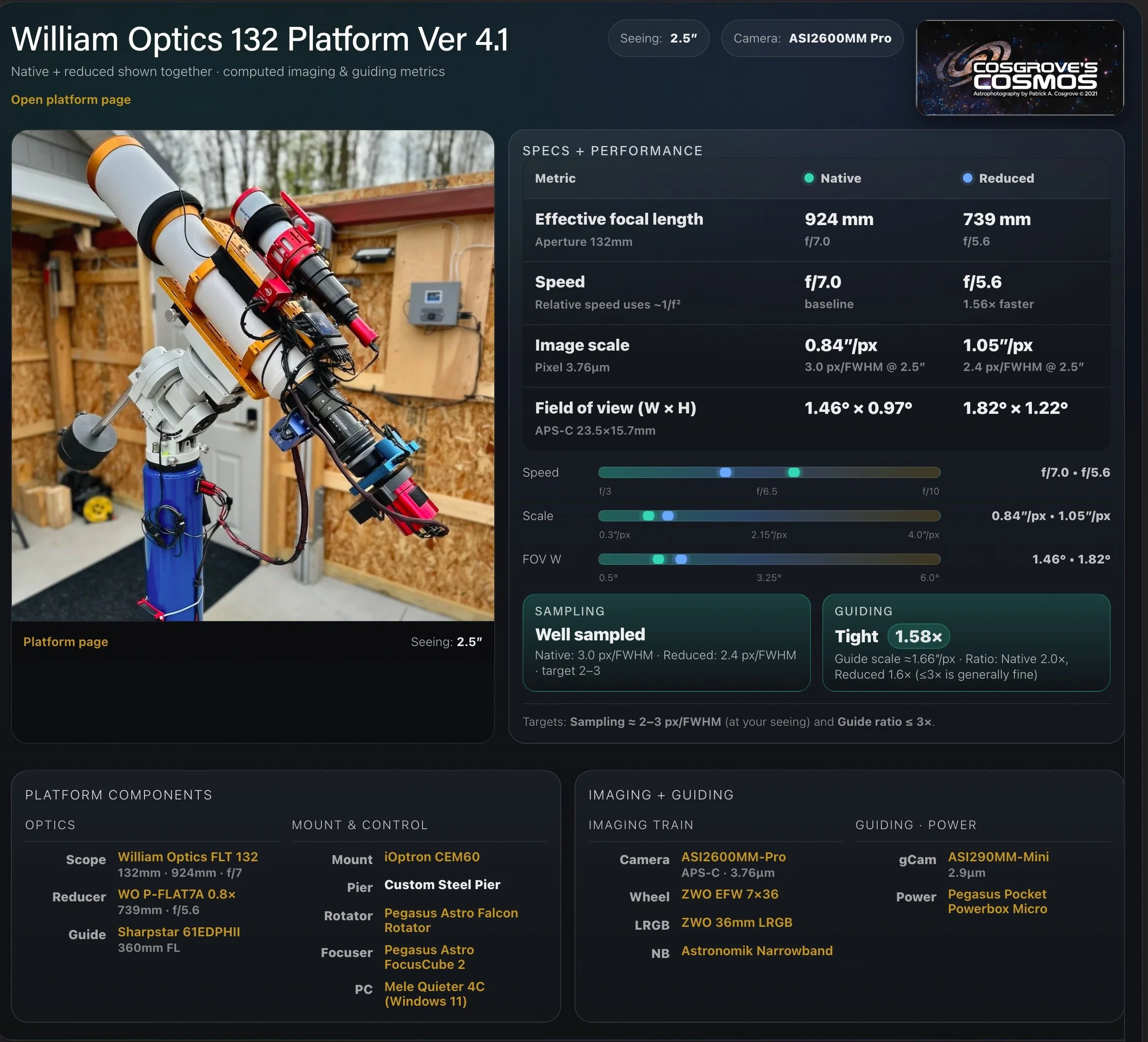
Platform used for this project
Software
Capture Software: PHD2 Guider, NINA
Image Processing: Pixinsight, Photoshop - assisted by Coffee, extensive processing indecision and second-guessing, editor regret and much swearing…..
Image Processing Walkthrough
(All Processing is done in Pixinsight, with some final touches done in Photoshop)
1. Blink
Ha
Blank 3 removed
Clouds 2 removed
Unsharp 1 removed
Tracking 2 removed
Some light clouds - not removed
Satellite trails - not removed
O3
Blanks 2 removed
In the Trees 3 removed
Clouds 6 removed
Tracking 2 removed
Thin clouds - not removed
S2
Blank 2 removed
Tracking 1 removed
In the Trees 1 removed
Clouds 5 removed
Red
In the Trees 2 removed
Clouds 1 removed
Green
In the Trees 3 removed
Clouds 1 removed
Darks
All good
Flats
All good
2. WBPP 2.8.9
Reset everything
Load all lights
Load all flats
Load all darks
Select - maximum quality
Reference Image - auto - the default
Set the output directory to a targeted wbpp folder
Pedestal value - set to auto
Darks -set exposure tolerance to 0
Lights - set exposure tolerance to 0
Lights - all set except for linear defect
Set for Autocrop
Executed in 1 hour and 26 minutes - no errors!
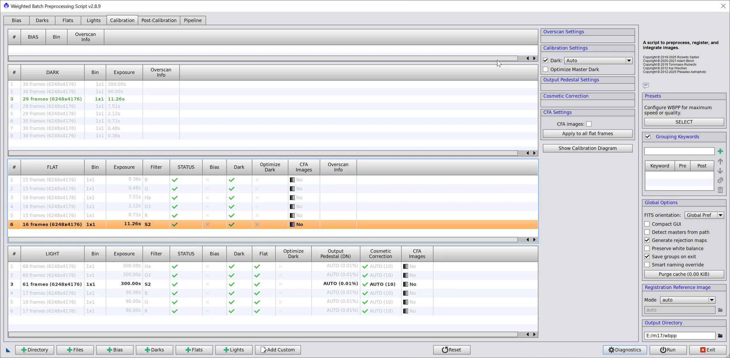
WBPP Calibration View
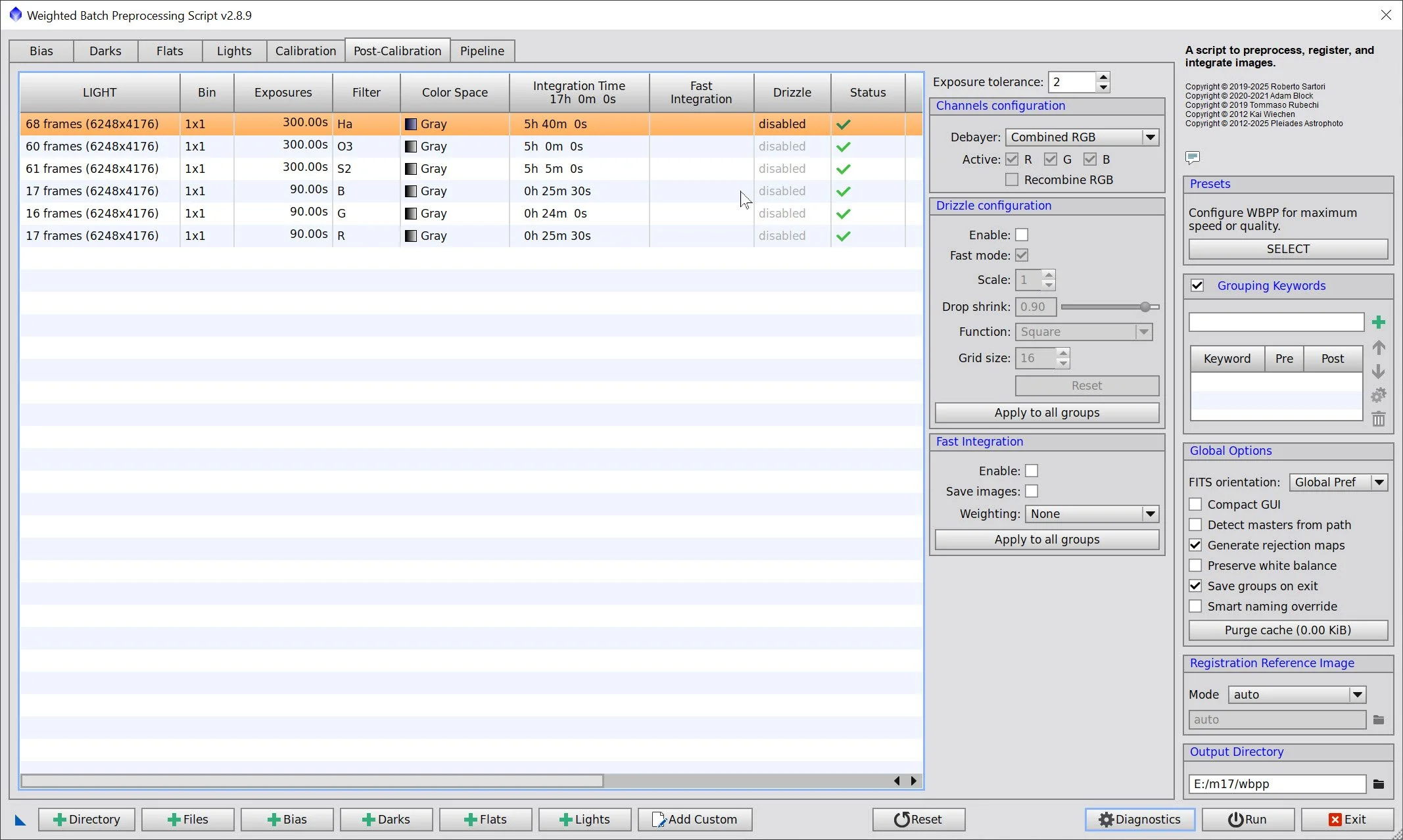
WBPP Post Calibration View
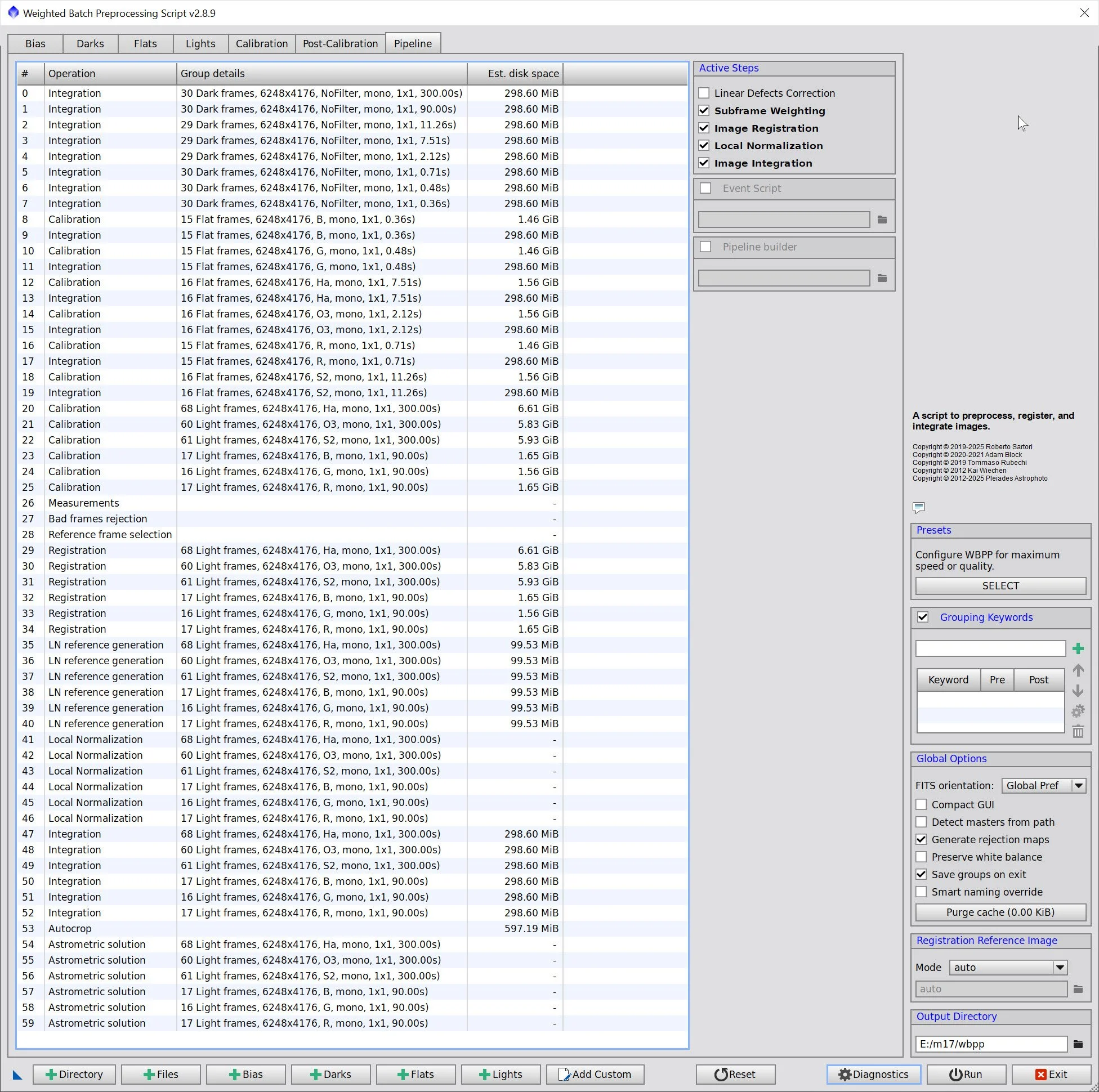
WBPP Pipeline View
3. Load Master Images
Load all master images and rename them.
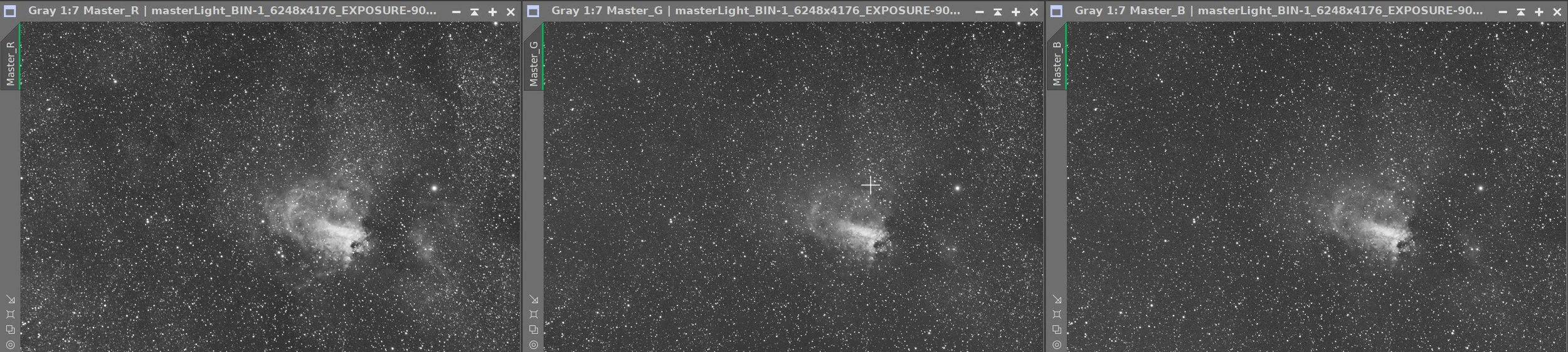
Master R, G, and B images

Maser Ha, O3, and S2 images
4. Process Linear RGB data
Create the RGB color image with the ChannelCombination tool
Run DBE on the linear color image:
Set up the sample pattern as shown
Fix with subtraction
Run SPCC and calibrate the color. Use the Sony 571 QE curve and ZWO RGB filters. See the panel setup below. Note that the regression results appear a bit unusual on one panel, but the resulting star images themselves appear satisfactory. Not sure what happened here, but I am happy with the result.
Run BXT correct-only. This will fix the stars. Not much to fix here, but I am just being careful.
Run default BXT - the stars are tight already, and I won’t be keeping starless images data.
Apply NXT to remove noise. NXT = 0.65
Use SXT with ‘Saving Stars’ (Unscreen Stars not selected as this is linear) to create RGB Stars and RGB Starless images. Set to a large sample box size
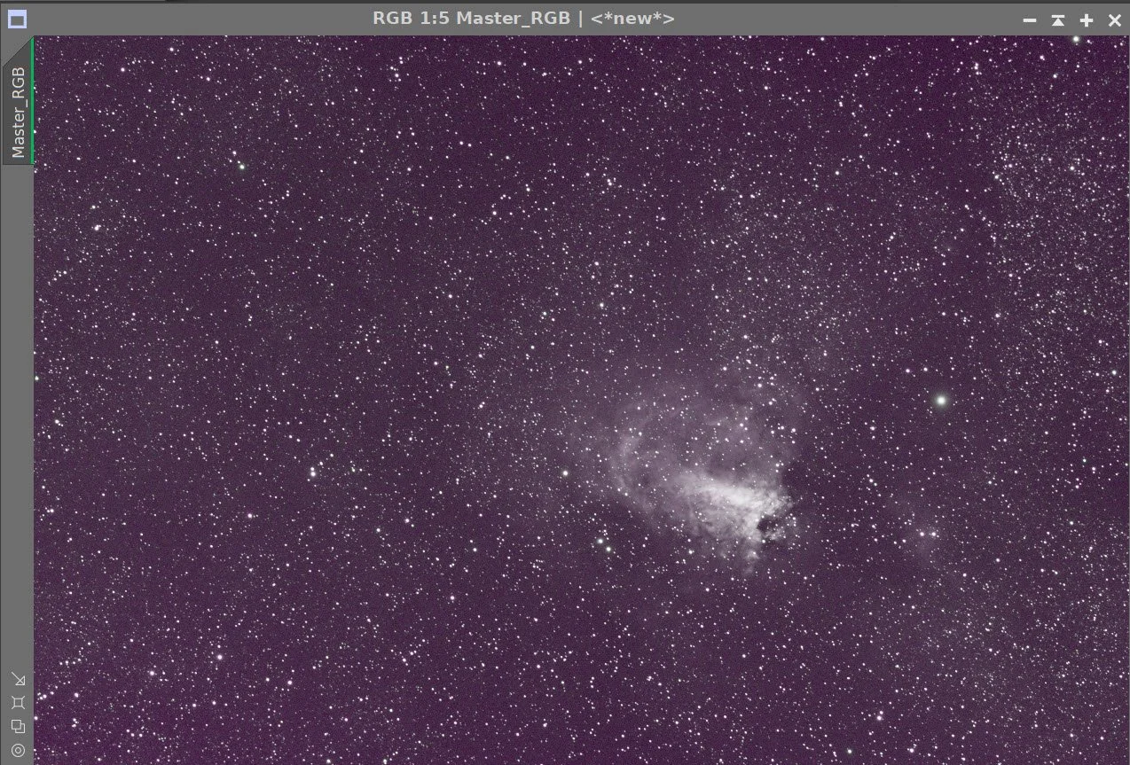
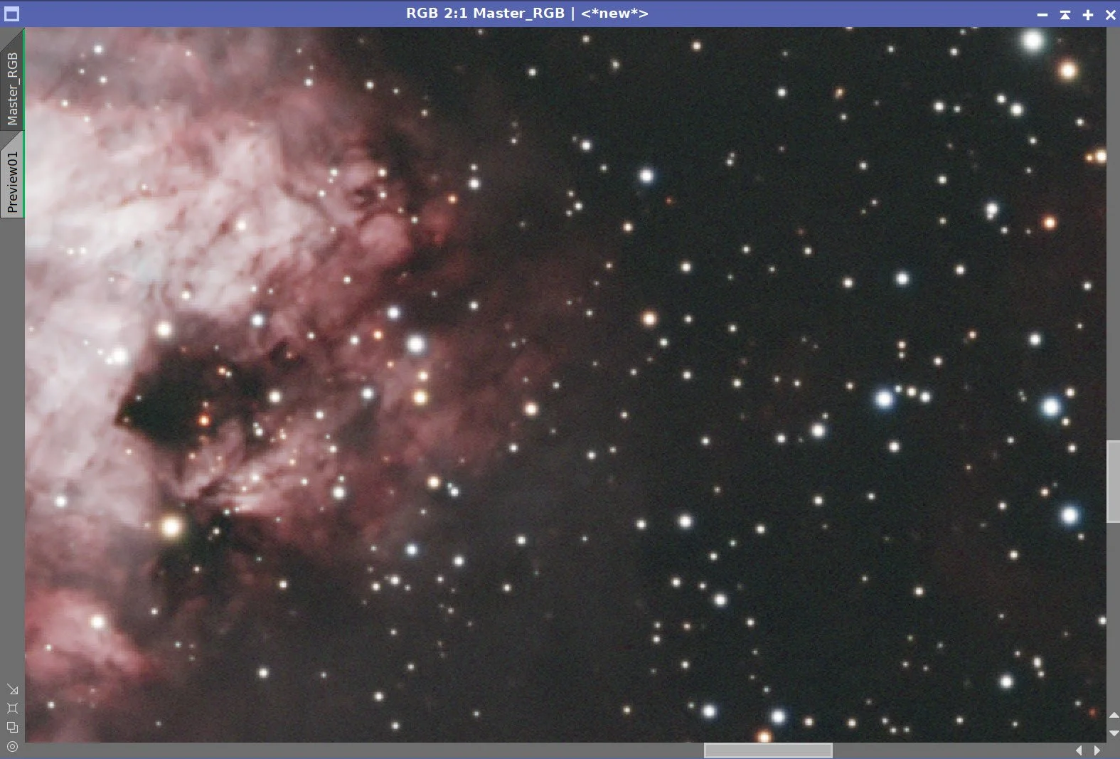
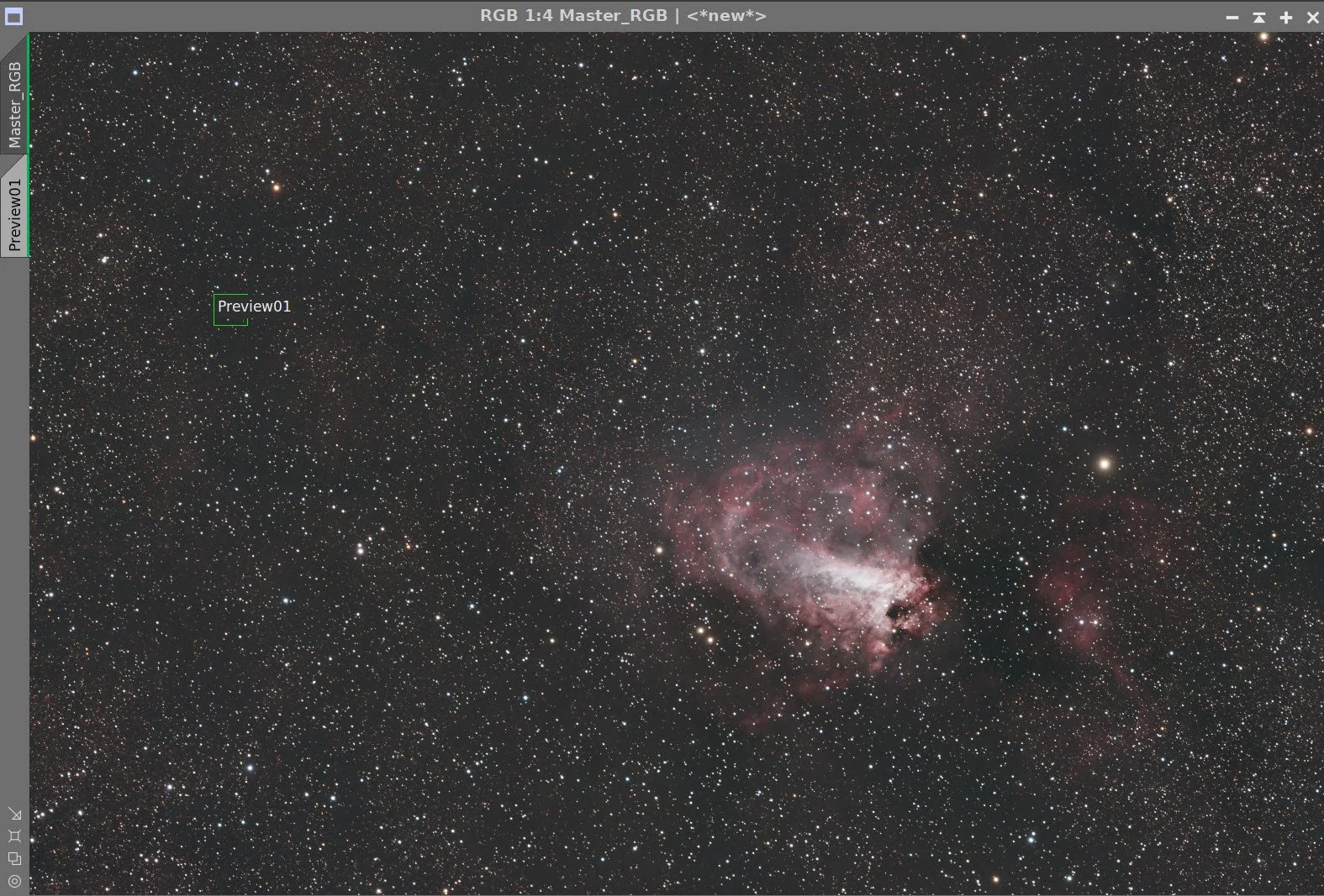
The initial RGB Linear Image.
Master RGB Sample Pattern (click to enlarge)
Master RGB Before DBE (click to enlarge)
Master RGB after DBE (click to enlarge)
Master RGB Background
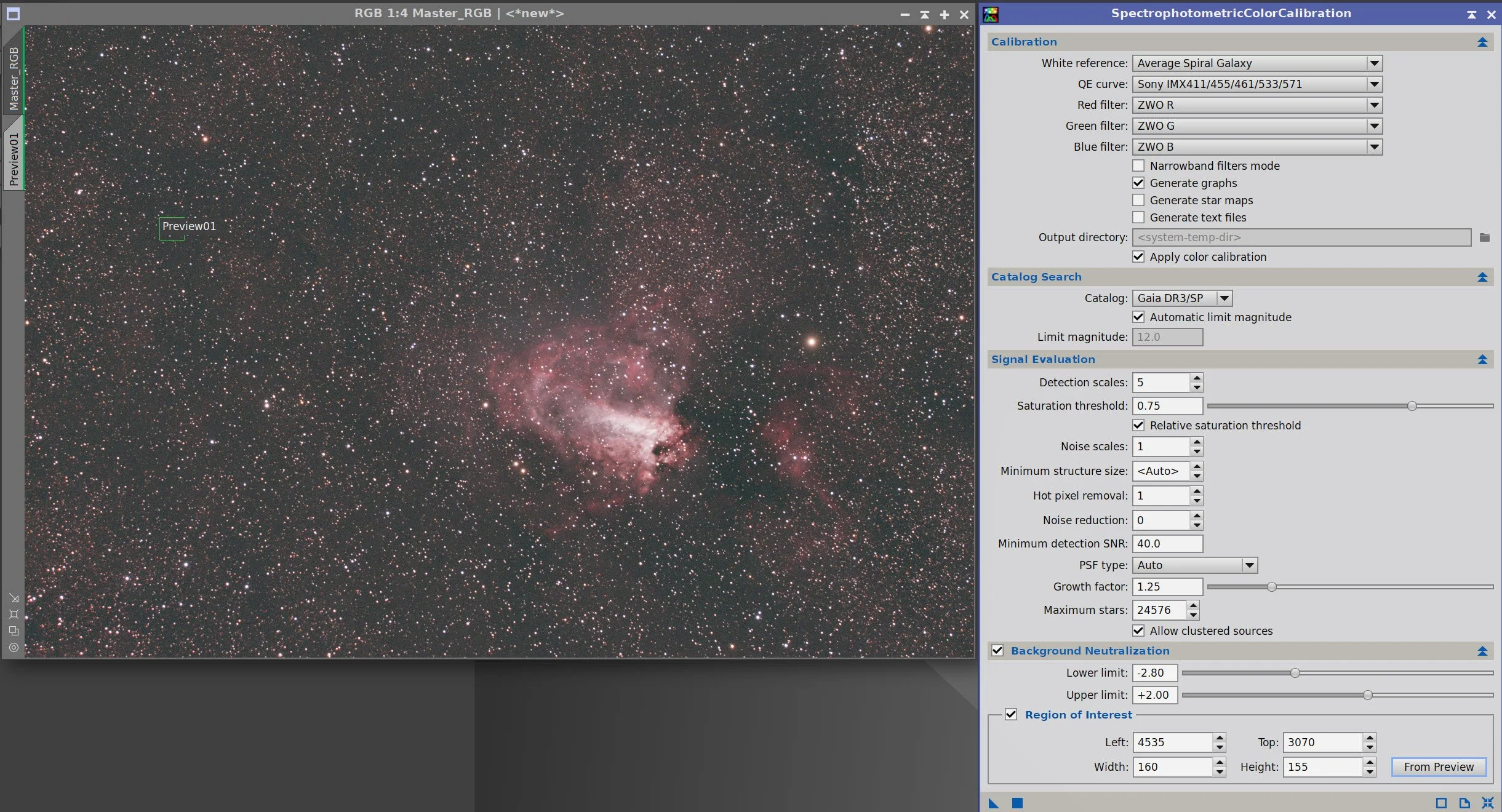
SPCC panel settings used.

The final regression result.
Master_RGB before SPCC run. (click to enlarge)
Master_RGB after SPCC run NOTE: The Paperclip Image is not a true object in outer space. It is a screen copy artifact (click to enlarge)


The Master RGB Image before BXT, After BXT Correction only, After BXT Full Correction, and After NXT = 0.65
Master_RGB before STX Star removal. NOTE: The Paperclip Image is not a true object in outer space. It is a screen copy artifact. (Sure it is… ah ha….)
RGB Stars Image resulting from STX. (click to enlarge)
5. Process the Linear SHO Color Image
Create the SHO Color image using the ChannelCombination Tool
Use NarrowbandNormalization to color-adjust the image. See the panel snap for parameters used.
This image is filled with nebulosity, and I don’t really see a gradient, so I am not going to run DBE.
The background has a lot of magenta in it. We will fix that with the following sequence:
Invert the image (magenta becomes green)
Run SCNR with Green at an amount = 0.9
Invert the image again.
Run BXT Correct Only - nothing much changes as the stars are already pretty round.
Run PFSImage to get star sizes. X = 2.18, Y= 2.05
Experiment with BXT settings for best results. I tend to use star sizes larger than what PFSImage finds.
Run BXT Full. See the panel shot below.
Apply NXT - 0.65
Take the image starless with SXT - use a large sample box - no need to save the stars - we will be using the RGB stars for this image!
The initial SHO color image (click to enlarge)
The normailized SHO image (click to enlarge)
After SCNR Green 0.9 (click to enlarge)
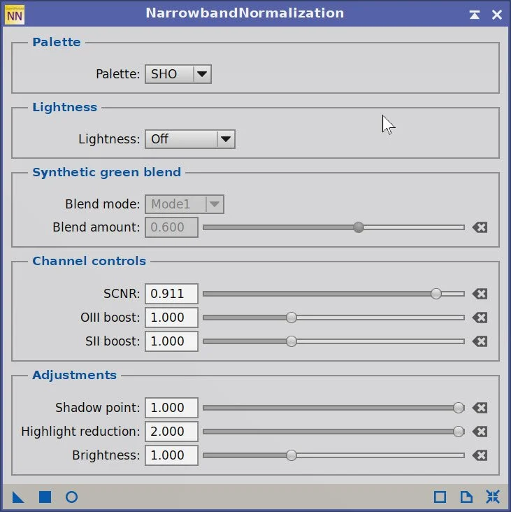
Params used to normalize the image.
Inverting th eimage. The magenta background is now green. (click to enlarge)
After another invert image. Magenta background is gone. (click to enlarge)

PFSImage results for Master

Final BXT Params used.

Master SHO Before BXT, After BXT Correct Only, BXT Full, and NXT = 0.65
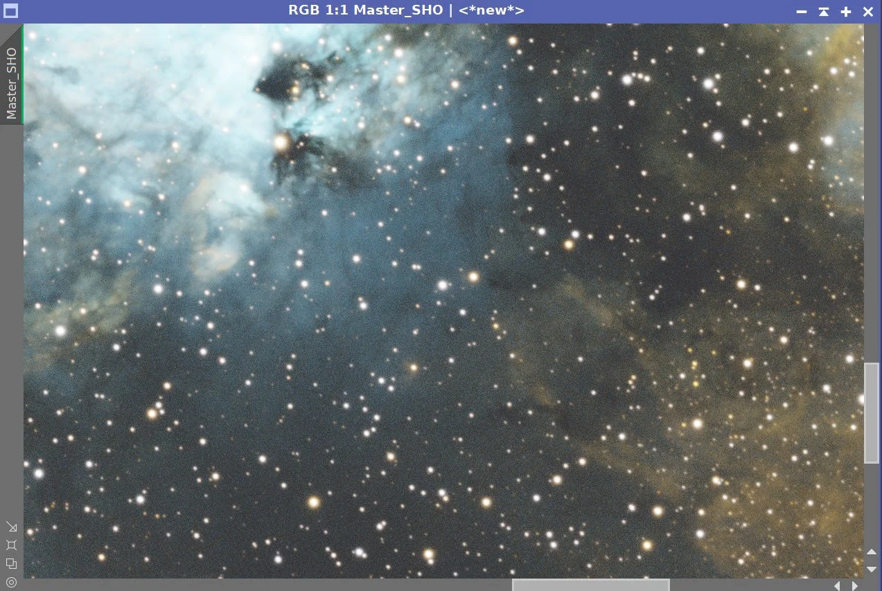
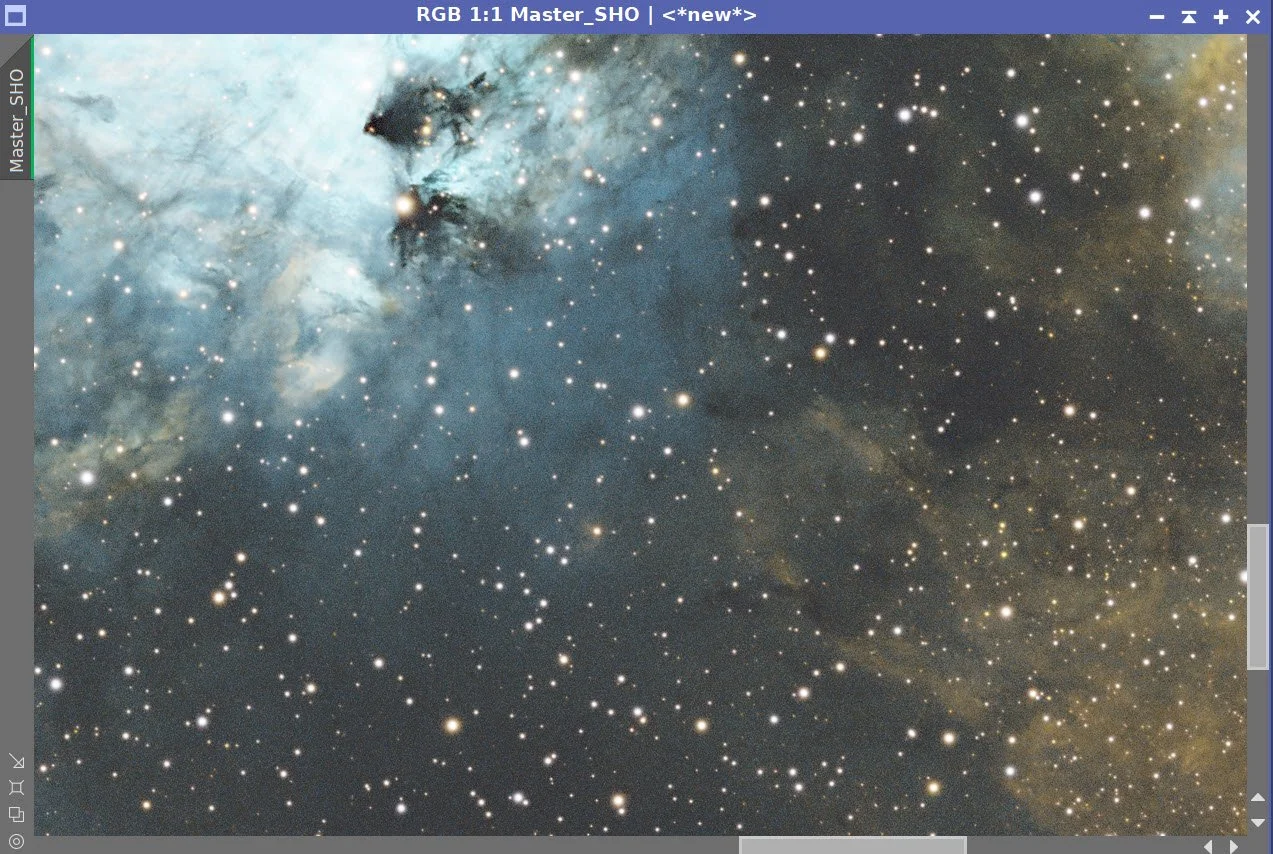
Master_SHO before Star Removal (click to enlarge)
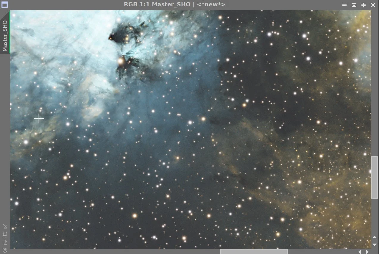
Master L Starless. (click to enlarge)
6. Move Images to the Nonlinear State
For RGB Stars, I used the Star Stretch by Seti Astro. Default parameters.
For SHO Starless, I used Statistical Stretch - also by Seti Astro. See panel snaps for parameters used.
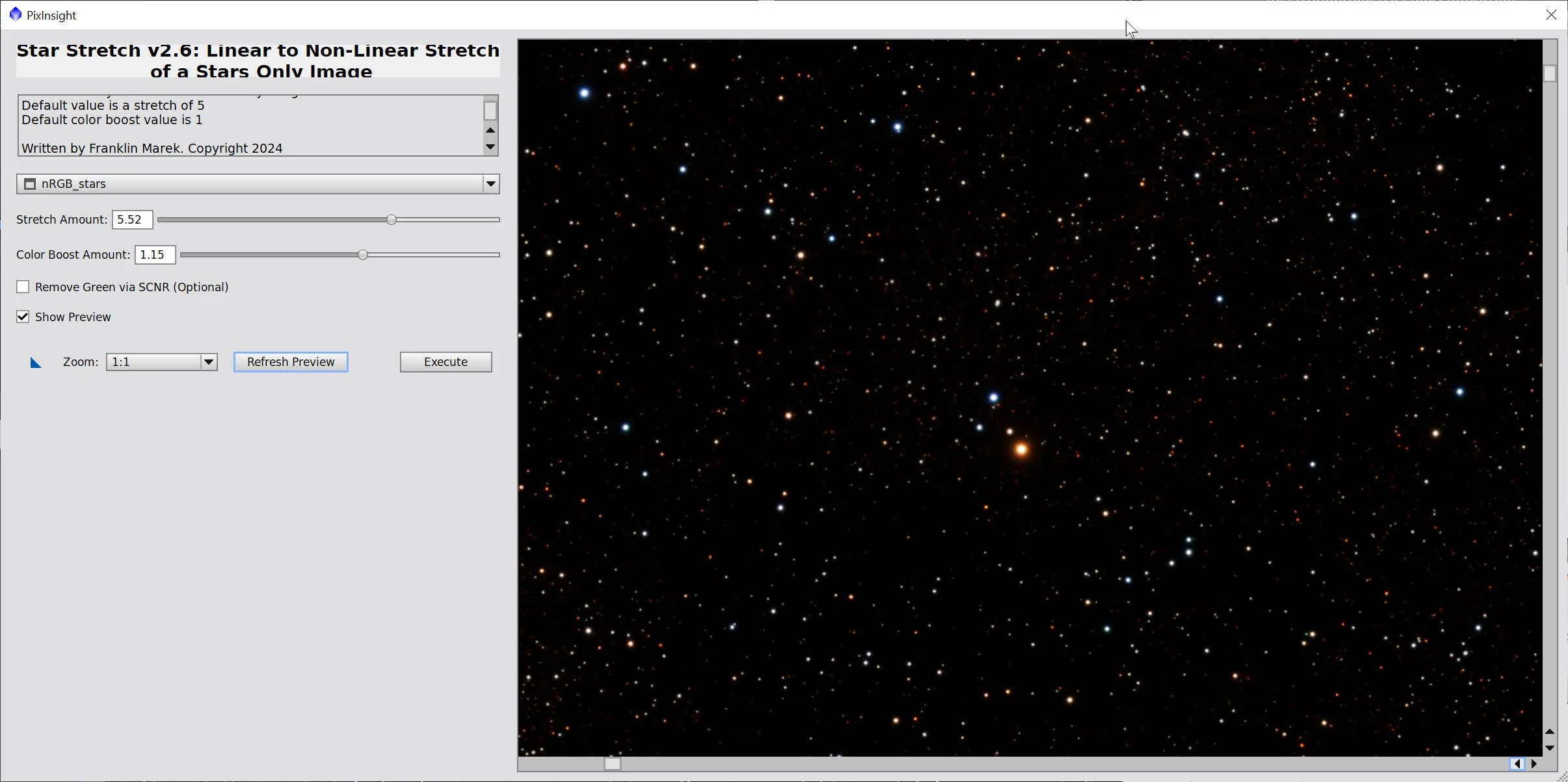
Stretch by Seti Astro used to take stars nonlinear.
Initial Nonlinear RGB Stars Image (click to enlarge)
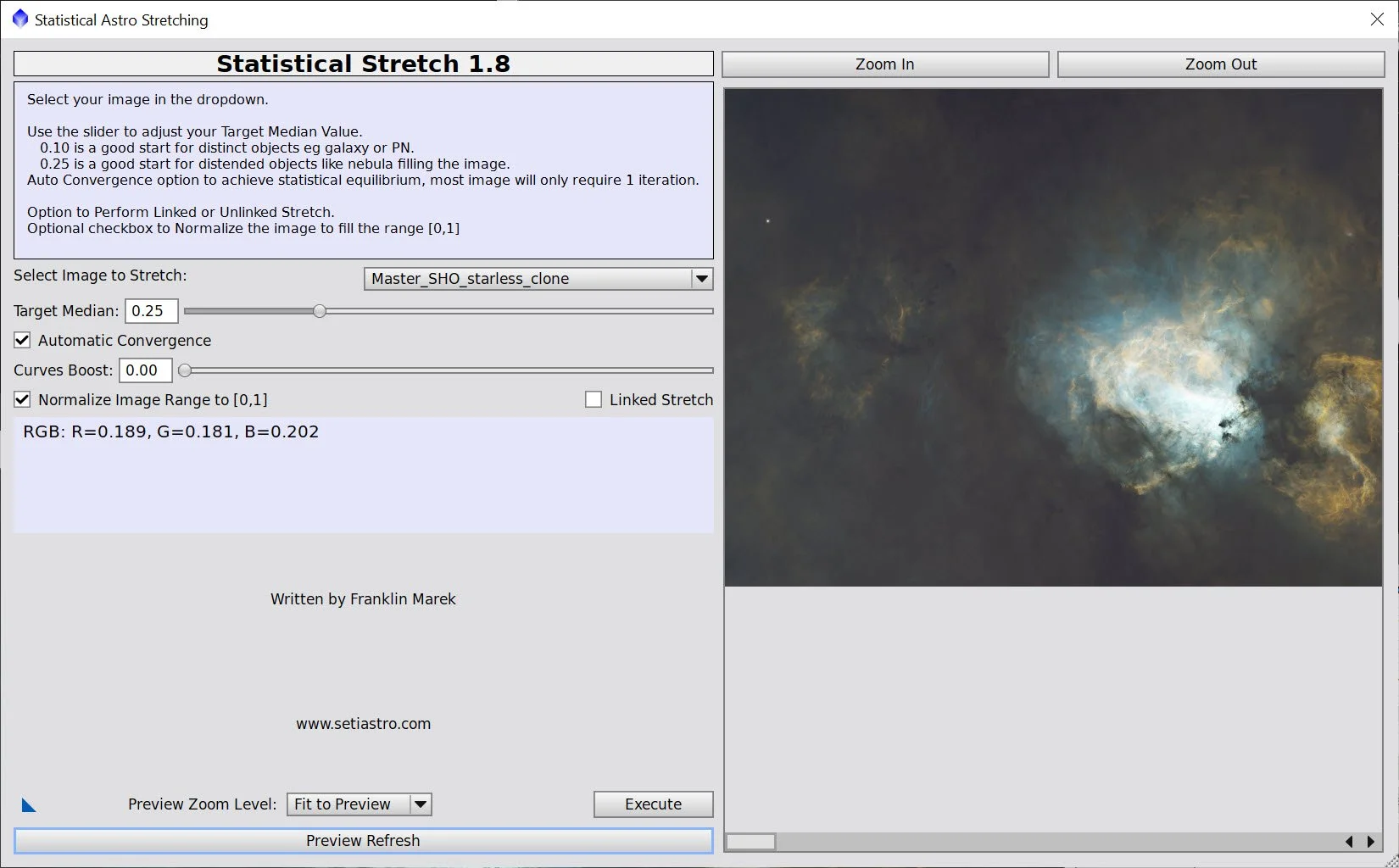
This set of params used on the SHO starless image.
Initial Nonlinear RGB Starless image (click to enlarge)
7. Process the Nonlinear RGB Stars Image
Simple - I used the CT tool to adjust brightness and Saturation until I was happy. Here is the final result.
Initial RGB Stars Image (click to enlarge)
9. Do the Processing of the Nonlinear SHO Starless Image
The core of the nebula is blocked out. So I ran HDRMT with levels = 8 with B3(s5)to bring this down a bit.
Perform a CT adjustment to improve the tone and colors.
At this point, I usually create a series of color masks and then adjust each key color I am interested in. This time, I used the free tool SelectiveColorCorrection. With this tool, you select a color, and it creates an internal mask for that color. Then, you can adjust almost every aspect of that color and see the results in the preview. This is the second time I used this tool, and I like it! I did a separate adjustment using this tool for Red, Blue, Cyan, Yellow, and shadows. The tool panel and parameters are shown below, along with the results of these changes.
At this point, I spent some time performing several Curve Transformations, refining the neutral tone scale, saturations, and making some color curve adjustments.
I had some feedback that the teal area might look better if it were bluer in color. So I created a Bluemask with the ColorMaskMod tool set to cover all cool tones. The resulting mask was then smoothed with Bill Blansan’s Mask Smoothing script.
The mask was applied, and the green curve was adjusted just a bit to rotate the color more towards blue.
Next - as a final touch - again based on some feedback - I decide to make the gold tones pop a bit more. I did this with the ColorSaturaton tool as shown below.
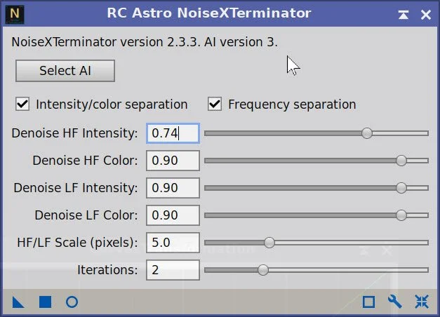
Finally, I did an NXT with the V3 parameters shown in the panel snapshot below. This was fairly aggressive, as the noise in the darker regions was amplified by all of the CT adjustments,
Do a final CT
The Initial SHO Image (click to enlarge)
After CT to adjust things (click to enlarge)
Selective Color Correction for Red - see params used. (click to enlarge)
SCC for Blue. (click to enlarge)
SCC for Cyan. (click to enlarge)
SCC for Yellow (click to enlarge)
SCC for shadows (click to enlarge)
After Several CT adjustments (click to enlarge)
After CT blue mask to shift blue area from teal to more a a blue. (click to enlarge)
After HDRMT with level = 8 (click to enlarge)
The resulting Change (click to enlarge)
After SCC for Blue (click to enlarge)
After SCC for Cyan (click to enlarge)
After SCC for Yellow (click to enlarge)
SCC for Shadows. (click to enlarge)
Blue Mask (clic to enlarge)
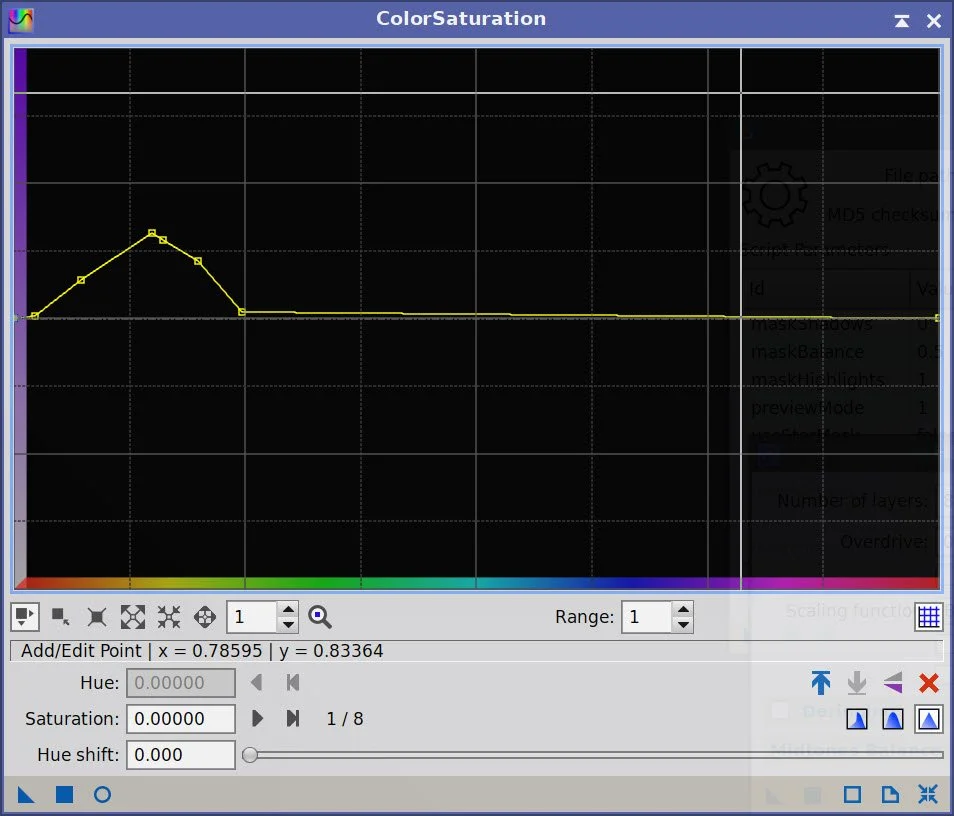
Color Boost for golden areas.

After Color_Saturation Adjust (click to enlarge)
Final version of the nL_starless image.
FInal Version of the nonlinear SHO Starless Image!
10. Combine the RGB Starless with the RGB Stars Image
Use the ScreenStars script to add the RGB Stars back in
The RGB Stars Image (click to enlarge)
The Final Starless LRGB image (click to enlarge)
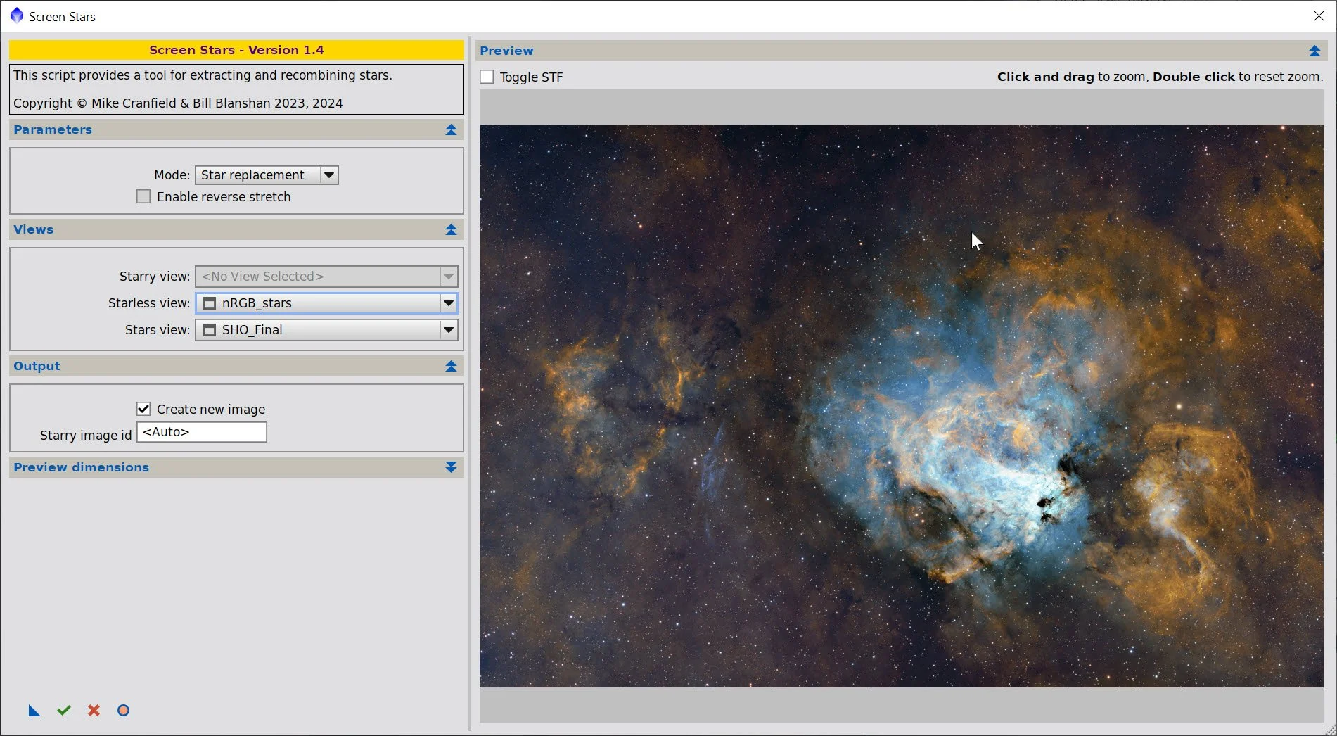
ScreenStars Panel Setup.
11. Export the Image to Photoshop for Polishing
Save the image as a TIFF 16-bit unsigned and move to Photoshop
Rotate the image 180 degrees - I think the image looks better this way.
Make tiny global adjustments with Clarify, Curves, and the Color Mixer
Added Watermarks
Export Clear, Watermarked, and Web-sized jpegs.

The Final Image!