
IC 5070 - The Pelican Nebula! 18.75 hours of SHO (my longest integration yet!)
Date: Sept 6, 2025
Cosgrove’s Cosmos Catalog ➤#0148
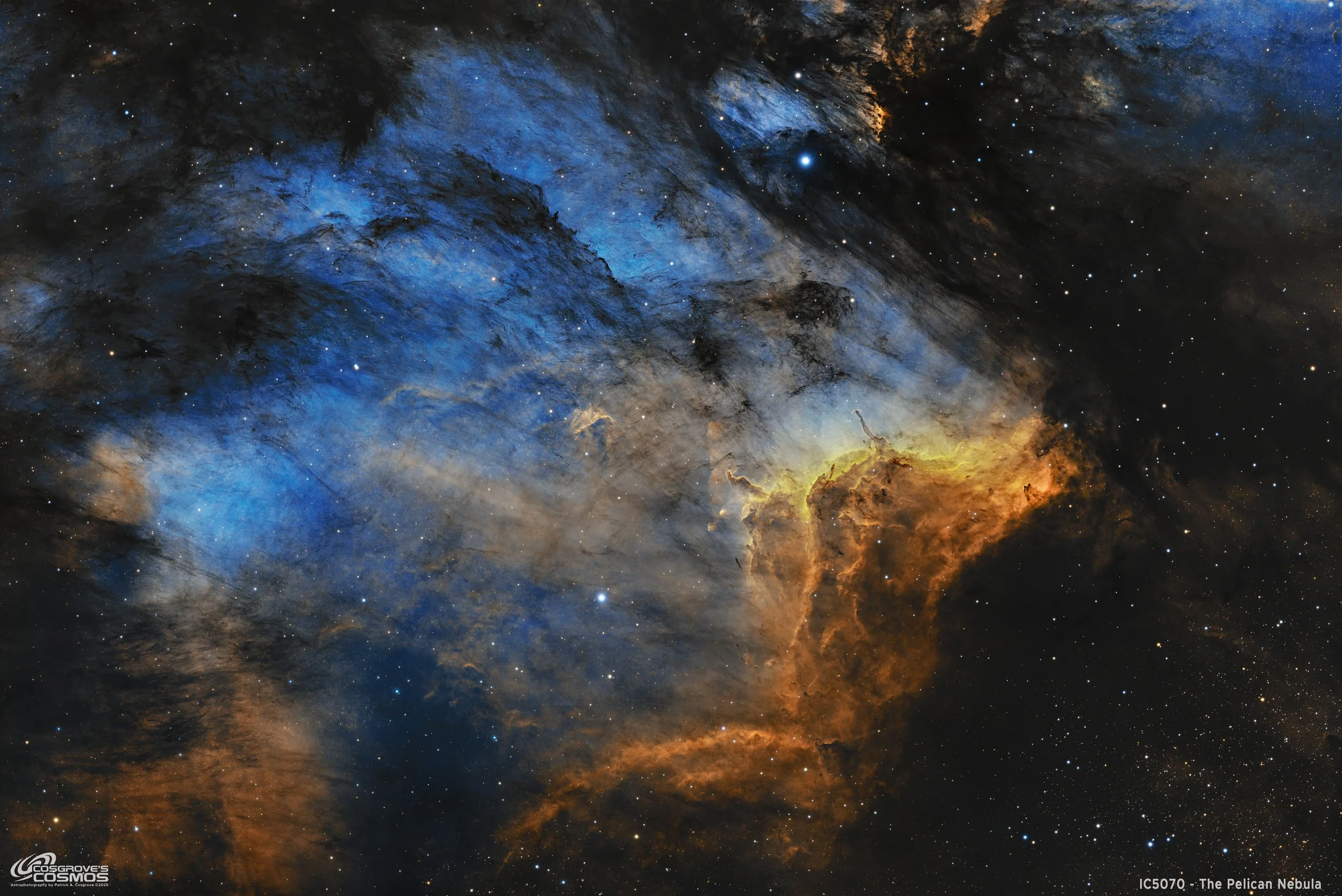
At almost 19 hours, this image of IC 5070 is my longest integration to date! (click image for hi-res version via Astrobin.com)
Granted Explore! Status on Flickr!

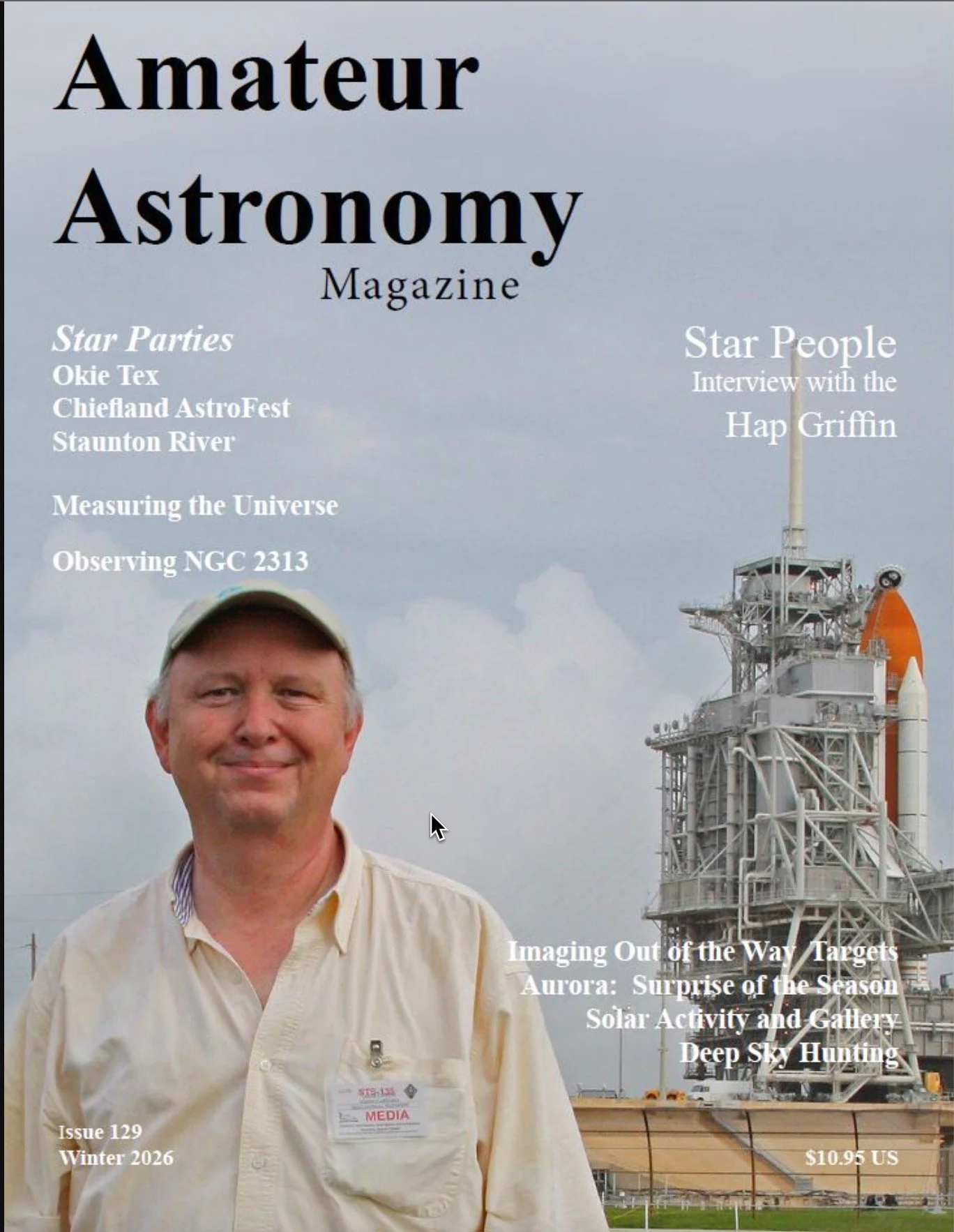
Amateru Astronomy Magazone, Winter 2026, Issues #129
Another image printed in the same issue - but here is the image description (click to enlarge)
The image and the annotated version (click to enlarge)
Table of Contents Show (Click on lines to navigate)
About the Target
The Pelican Nebula (IC 5070) is a bright emission nebula found in the constellation of Cygnus. It is physically part of the same cloud complex as the North America Nebula (NGC 7000). A foreground dark cloud (Lynds Dark Nebula LDN 935) creates the visual gap between these two well-known targets.
Modern Gaia-based studies place the complex at roughly 2,600–2,700 light-years away (older sources often quoted ~1,800 light-years).
The Pelican spans roughly 60′ × 50′ and lies near the bright star Deneb, though Deneb is not the ionizing source.
History
IC 5070 and the adjacent bright ridge IC 5067 were added in John L. E. Dreyer’s Second Index Catalogue (IC II, 1908), part of his supplements to the NGC that incorporated many photographic-plate-enabled discoveries.
In 1959, Stewart Sharpless recognized that the North America and Pelican Nebulae are parts of a single H II complex (Sh2-117), and Westerhout’s 1958 radio survey listed the region as W80. Early speculation that Deneb powered the nebula has since been rejected. In 2005, Comerón & Pasquali identified a heavily reddened O5 V star (2MASS J205551.3+435225) behind LDN 935 as the main ionizing source. Gaia EDR3 later refined the distance and kinematics of this star, cementing its link to the complex.
Interesting Details & Aspects
A standout feature is the curved, bright ionization front along the “neck” of the Pelican, cataloged as IC 5067; APOD notes this ridge spans ~10 light-years and outlines the head/neck profile. The broader W80 region extends ~3° across in radio/optical maps, making it a large, nearby laboratory for star-formation studies.
The Science
The Pelican is a stellar nursery. Intense ultraviolet radiation from the embedded O-type ionizing source drives an advancing ionization front into surrounding molecular gas, sculpting pillars and globules and triggering new star formation along their edges. Numerous young stellar objects and Herbig–Haro jets are present—famously HH 555 in IC 5067—direct evidence of ongoing protostellar outflows. The region is considered relatively evolved (low overall density, lacking ultracompact H II pockets) but continues to form low and intermediate-mass stars.
Annotated Image
Created in Pixinsight using the ImageSolver and AnnotateImage scripts.
The Location in the Sky

This annotated image created with Imagesolver and FInderChart Scripts in Pixinsight.
About the Project
Picking the Target
In preparing for this past New Moon cycle, I was hunting for possible targets.
Cygnus was now prominent in the sky, and this region is rich in interesting targets. Over the past few years, I have shot a lot of targets there.
As I scanned through some charts, I noticed that the Pelican Nebula was in a favorable position in the sky. At the time, I was not really interested in shooting the Pelican Nebula again as I had already shot it twice before, and my second one, I thought, was quite good.
But I thought there might be some overlooked targets in the neighborhood that I could go after, so I was "scoping’ the area once again.
As part of this, I looked at my most recent shot of the Pelican. It was taken about 5 years ago, and as I looked at it again, my reaction was: “Hmm - this isn’t so great after all - I can do better than that!”
Over time, you evolve in your standards and processing preferences. I hadn't really looked at this image for a while, and I suppose I don't see it the same way now as I did back then.
Back then, I was super proud of it. Now - ehhh - not so much!
I decided then and there that I would try one more time to see if I could improve upon my previous results.
The First Attempt
The first time I shot the Pelican was in September of 2019 - a few months after I first started doing astrophotography.
You can read bout that project HERE.
This was a 2.6-hour integration using my first OSC camera on my William Optics 132mm FLT scope. At the time, I could not even see enough detail to understand how the Pelican Nebula had gotten its name!
The Second Attempt
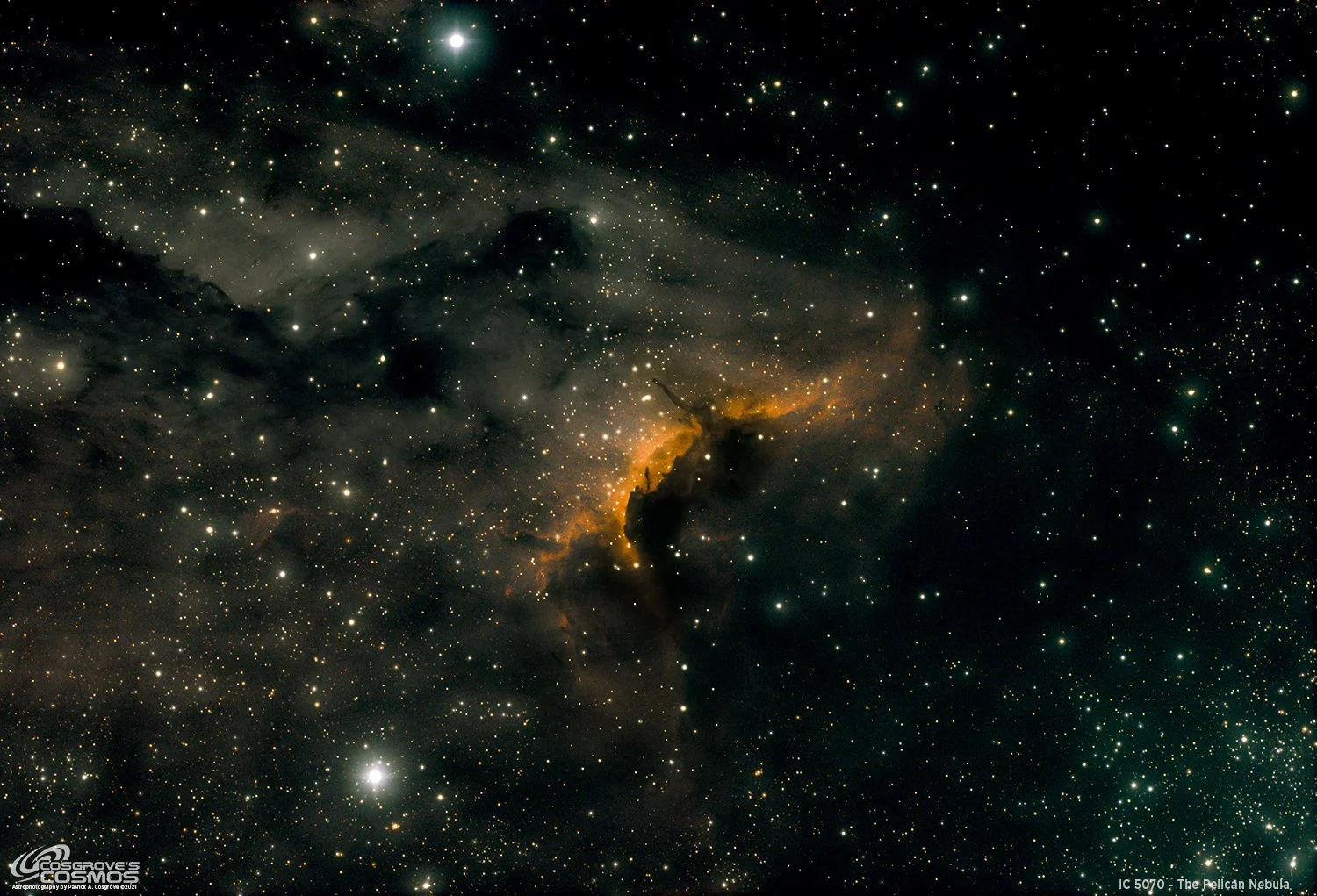
The second time I shot it was in October of 2020 - about a year later.
This is the one I was so proud of. By this time, I had my Astro-Physics 130mm f/8.35 scope up and running and was using my first Mono camera.
This project can be seen HERE. This image was the result of 3.4 hours of SHO integration.
Here are both images so you can compare them side by side.
M First Attempt at IC 5070 in 2019. (click to enlarge)
My second attempt in 2020 - this is the one I “was” proud of! (click to enlarge)
I planned on using the Williams Optics 132mm scope with the 0.8 reducer. This would give me a slightly wider field with faster f/5.5 optics. It would be a narrowband image, and I would now be shooting from my new observatory. That meant that I could go after more marginal nights and see how much time I could rack up before the Moon got in the way again.
Data Collection
Data was collected on the nights of August 22, 24, 30, and 31, 2025.
This was at the end of the month, so the nights were finally getting longer and cooler. If you looked at the weather apps, none of these nights looked very promising. But one member of our local group, Gary, is a weather wizard. Gary was giving us nightly updates on conditions as he saw them, and trusting in Gary, I set up for each night and hoped for the best.
Gary was pretty accurate in his predictions, and over the course of these 4 nights, I captured a total of 21 hours’ worth of data! This is the most I have ever collected on a single target.
However, the nights were not perfect. Thin clouds were coming through at times — not enough to lose guiding - but enough to ruin a frame.
I blinked all of the images and ended up removing about 2 hours of frames that were badly attenuated by the clouds. This still left me almost 19 hours of good data.
Shots were 300 seconds long with the camera cooling set to -10 degrees C. I usually run at -15 °C, but the hot weather was such that the camera could not achieve that temperature, so I have been running at -10 °C in case we have another warm night.
I shot only narrowband images. Lately, I have been collecting RGB data to have natural color stars. This time, I want to try out some of the scripts out there that claim to make narrowband stars look more normal. I will see how that works out!
All new cal frames were shot on September 2.
Processing Overview
This was a bright nebula target, and as such, I did not feel it needed drizzle processing.
The processing done was straightforward and followed my standard workflow for SHO images, which is outlined below.

My typical SHO Starless Workflow.
This was one of those images that was easy to process.
I followed my standard workflow and created three color masks, which proved very useful.
I created a Warm Tone Mask, which I used to adjust the gold-colored areas. I adjusted the color, the saturation, and the brightness. There is a lot of detail located in these regions, so I also used LocalHistogramEqualization to enhance both small-scale and large-scale features found there.
A Cool Tone Mask was used just for color adjustments.
A Yellow Mask was used to adjust the bright yellow line on one side of the Pelican’s neck.
I used Seti Astro’s NB-to-RGB Star script to clean up narrowband stars. That seemed to work reasonably well, and I think the resulting stars looked fine.
I have found that sometimes a strong nebula requires larger stars so they don’t get lost. So I created star images with various-sized stars and decided which worked best with the starless image. In this case, it was the larger star sizes.
I wrestled with whether I should rotate the image or not. If I rotated it, I would end up with a heads-up Pelican:

I considered rotating the image to look like this, but ultimately used the original framing.
Ultimately, I opted for the original framing.
Look below for the complete step-by-step walkthrough of the processing. Note: This walkthrough is based on Pixinsight.
Final Results
I was a little stunned by how much more detail and the sharpness I was able to capture here. I love the final image and feel that I have clearly improved on my previous efforts.
It also demonstrated to me the value of shooting from an observatory. I captured data on nights I might have skipped in the past, as they looked marginal.
I believe that having a consistent setup and polar alignment enabled me to capture finer details than I had before.
More Information
🌌 Target Details
https://en.wikipedia.org/wiki/Pelican_Nebula — Overview of IC 5070: location in Cygnus, relationship to NGC 7000, size, and basic properties.
https://simbad.cds.unistra.fr/simbad/sim-id?Ident=IC%205070 — SIMBAD object page with identifiers, coordinates, literature links, and catalogs for IC 5070.
https://noirlab.edu/public/news/noao0314/ — NOIRLab news note describing the Pelican–North America (W80) complex and the ionization front context.
https://apod.nasa.gov/apod/ap160526.html — APOD on IC 5067 (the Pelican’s “neck” ridge) with a concise caption about the region.
📜 History & Catalogs
https://cseligman.com/text/atlas/ic50a.htm — Historical notes and DSS views for IC entries, including IC 5070 (Pelican Nebula).
https://en.wikipedia.org/wiki/New_General_Catalogue — Background on the NGC and Dreyer’s Index Catalogue,s where IC 5070 was listed.
https://en.wikipedia.org/wiki/North_America_Nebula — History of the neighboring NGC 7000 and its linkage to the Pelican as one cloud, with classic references.
🔬 Science & Research
https://www.aanda.org/articles/aa/abs/2005/05/aa1788/aa1788.html — A&A paper identifying the main ionizing O-type star for the North America/Pelican complex.
https://arxiv.org/abs/2012.05074 — Gaia EDR3 study refining distance and motion for the complex’s ionizing source.
https://arxiv.org/abs/1102.0573 — Spitzer MIPS/IRAC survey cataloging thousands of YSO candidates in the North America/Pelican region.
https://www.jpl.nasa.gov/images/pia13845-north-america-nebula-in-different-lights/ — JPL page comparing visible/IR views; explains dust, star formation, and what IR reveals here.
💡 Interesting Facts & Features
https://apod.nasa.gov/apod/ap111126.html — APOD close-up of the Pelican with notes on dark pillars and active star formation.
https://www.jpl.nasa.gov/news/new-view-of-family-life-in-the-north-american-nebula/ — Brief article on star-formation “life stages” seen in this complex.
https://commons.wikimedia.org/wiki/File:Herbig-Haro_555.png — Annotated view highlighting HH 555 jets embedded in the Pelican’s “neck.”
https://www.nasa.gov/image-article/swirling-landscape-of-stars/ — NASA image article describing clusters of very young stars and dust structures in the area.
🔭 Observing & Imaging Guides
https://www.astronomy.com/observing/101-must-see-cosmic-objects-the-north-america-nebula/ — Practical overview of the larger complex with observing pointers relevant to the Pelican.
https://www.skyatnightmagazine.com/astrophotography/nebulae/north-america-nebula-ngc-7000 — Imaging/observing tips for the North America/Pelican region.
https://in-the-sky.org/data/catalogue.php?cat=IC&type=HII — Catalog listing with IC 5070 among Cygnus H II regions, useful for quick lookup and finder info.
https://esahubble.org/projects/fits_liberator/fitsimages/todd_nolan_3/ — ESA/Hubble page with a high-resolution processed image of the North America/Pelican field for reference framing.
Capture Details
Lights Frames
Taken the nights of August 22, 24, 30, and 31, 2025
81 x 300 seconds, bin 1x1 @ -10C, Gain 100, Astronomiks 6nm Ha Filter - 36mm unmounted.
73 x 300 seconds, bin 1x1 @ -10C, Gain 100, Astronomiks 6nm O3 Filter - 36mm unmounted.
71 x 300 seconds, bin 1x1 @ -10C, Gain 100, Astronomiks 6nm S2 Filter - 36mm unmounted.
Total - after culling bad subs - of 18 hours and 45 minutes.
Cal Frames
30 Darks at 300 seconds, bin 1x1, -10C, gain 100
30 Dark Flats at Flat exposure times, bin 1x1, -10C, gain 0 for RGB and gain 100 for narrowband
One set of Flats done:
15 Ha Flats
15 O3 Flats
15 S2 Flats
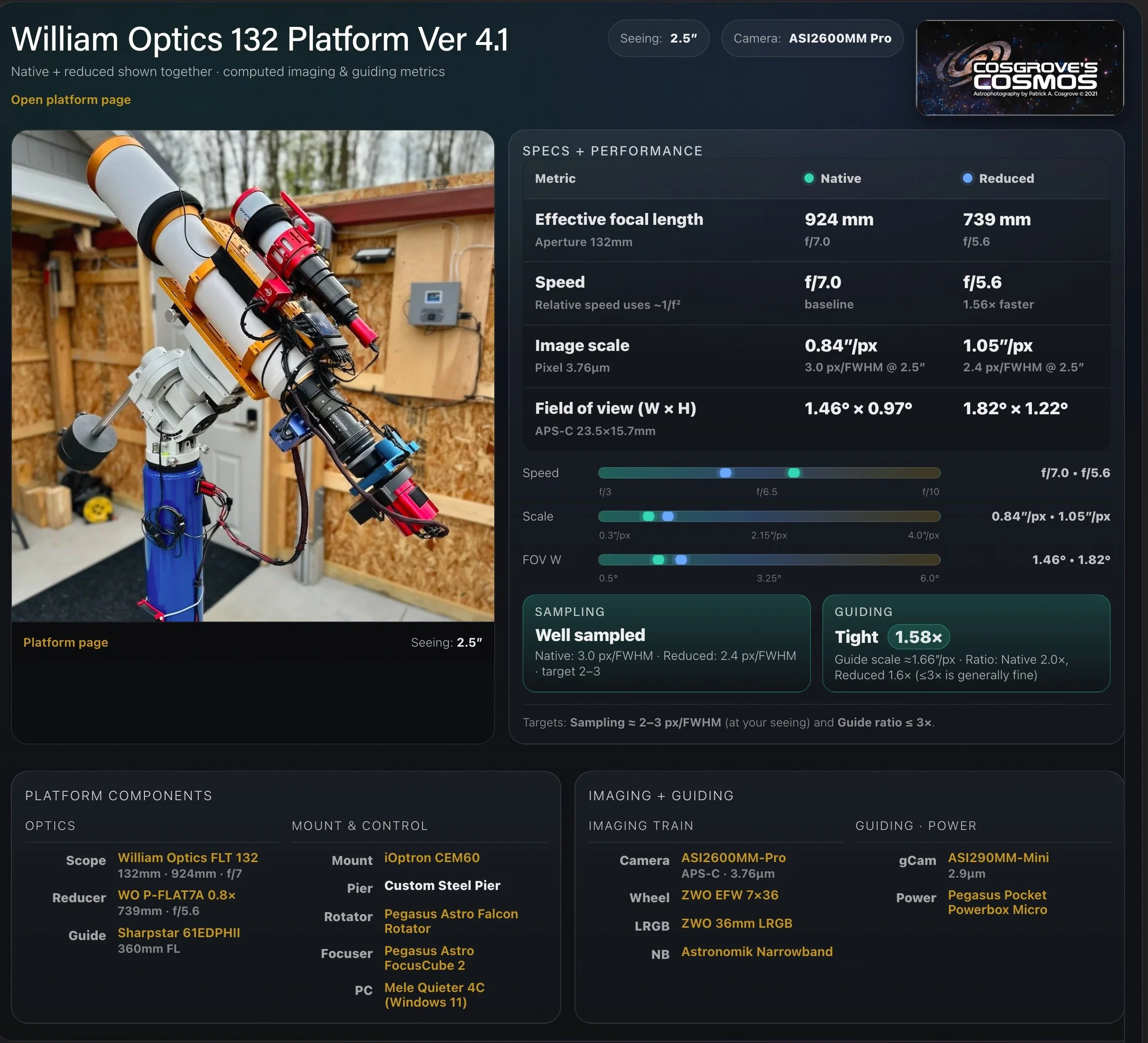
Platform used for this project
Software
Capture Software: PHD2 Guider, NINA
Image Processing: Pixinsight, Photoshop - assisted by Coffee, extensive processing indecision and second-guessing, editor regret and much swearing…..
Image Processing Walkthrough
(All Processing is done in Pixinsight, with some final touches done in Photoshop)
1. Blink
Ha
4 removed due to clouds
Satellite trails - not removed
O3
10 removed due to clouds
S2
12 removed due to clouds
Darks
All good
Flats
All good
Summary
26 frames lost for a total of 2.16 hours!
2. WBPP 2.8.9
Reset everything
Load all lights
Load all flats
Load all darks
Select - maximum quality
Reference Image - auto - the default
Set the output directory to a targeted wbpp folder
Pedestal value - set to auto
Darks -set exposure tolerance to 0
Lights - set exposure tolerance to 0
Lights - all set except for linear defect
Set for Autocrop
Executed in 1 :02:07 - no errors!

WBPP Calibration View

WBPP Post Calibration View
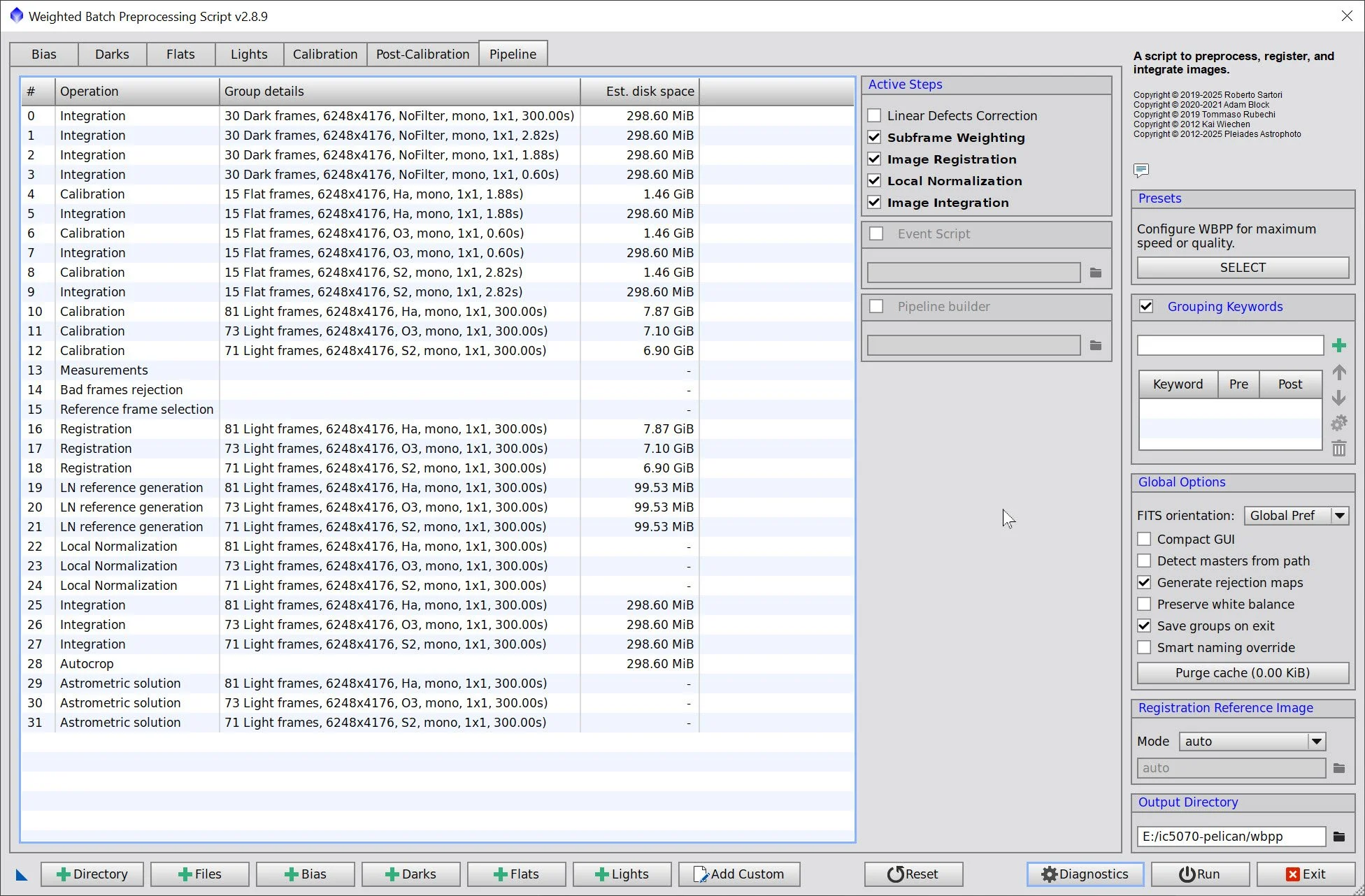
WBPP Pipeline View
3. Load Master Images
Load all master images and rename them.

Maser Ha, O3, and S2 images
4. Create and Process the SHO Color Image
Using the ChannelCombination Tool, create the first SHO color image.
This image has a lot of nebulosity, and I am not sure there is much of a gradient at this point, so I did not do a DBE operation here as I normally would.
I applied BXT Correct-Only to clean up the stars - not really much to clean up here.
Then I ran PFSImage to measure star sizes. In this case, they were X = 1.85 and Y = 1.73.
Experimenting with various params, I chose the configuration I wanted on BXT and ran the full version of that. I find I get the best results if I go 25-33% larger than what is measured by PFSImage - in this case, 2.74. See the screensnap below for details.
Then I experimented with NXT. There is remarkably little noise in this image, but I did run NXT - see the screensnap below for the parameters used.
Now use SXT to remove the stars. Save the star images. No need to unscreen.
The starless image does seem ot have a bit of gradient going from the bottom right to the upper left. I decided to try to use the Seti Astro AutoDBE tool on it. I mapped out exclusion zones and then ran it. Seemed to work OK.
Finally, use NarrowbandNormalization to get the color right. See the params used below.
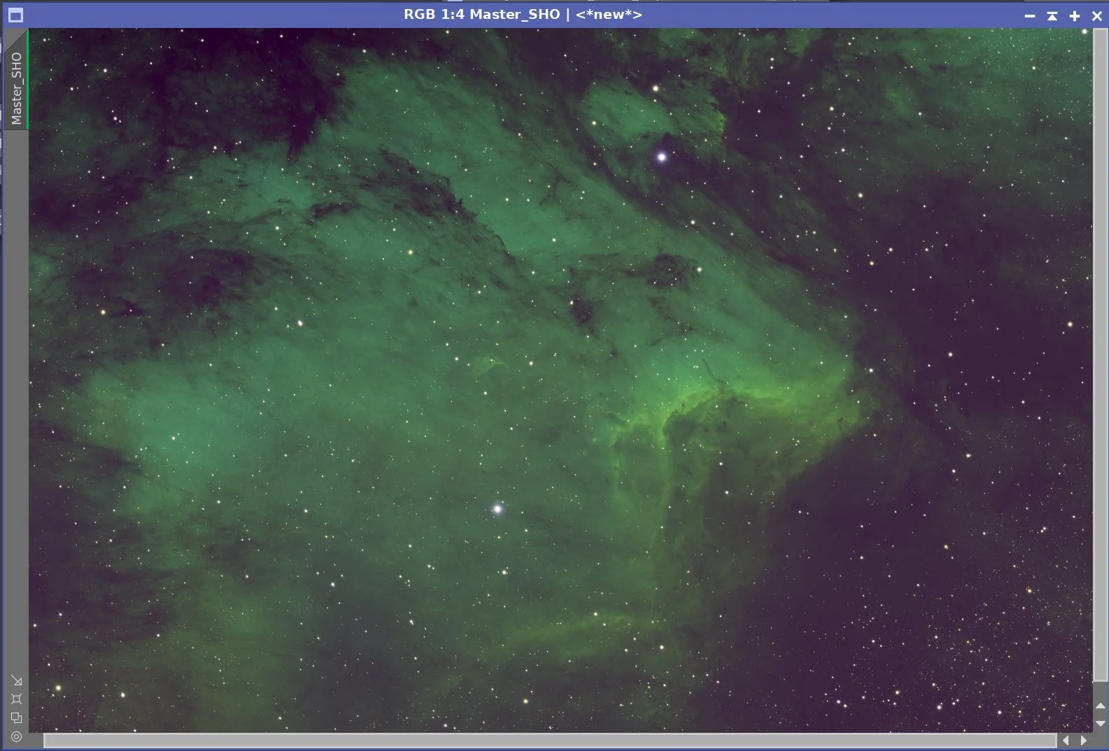
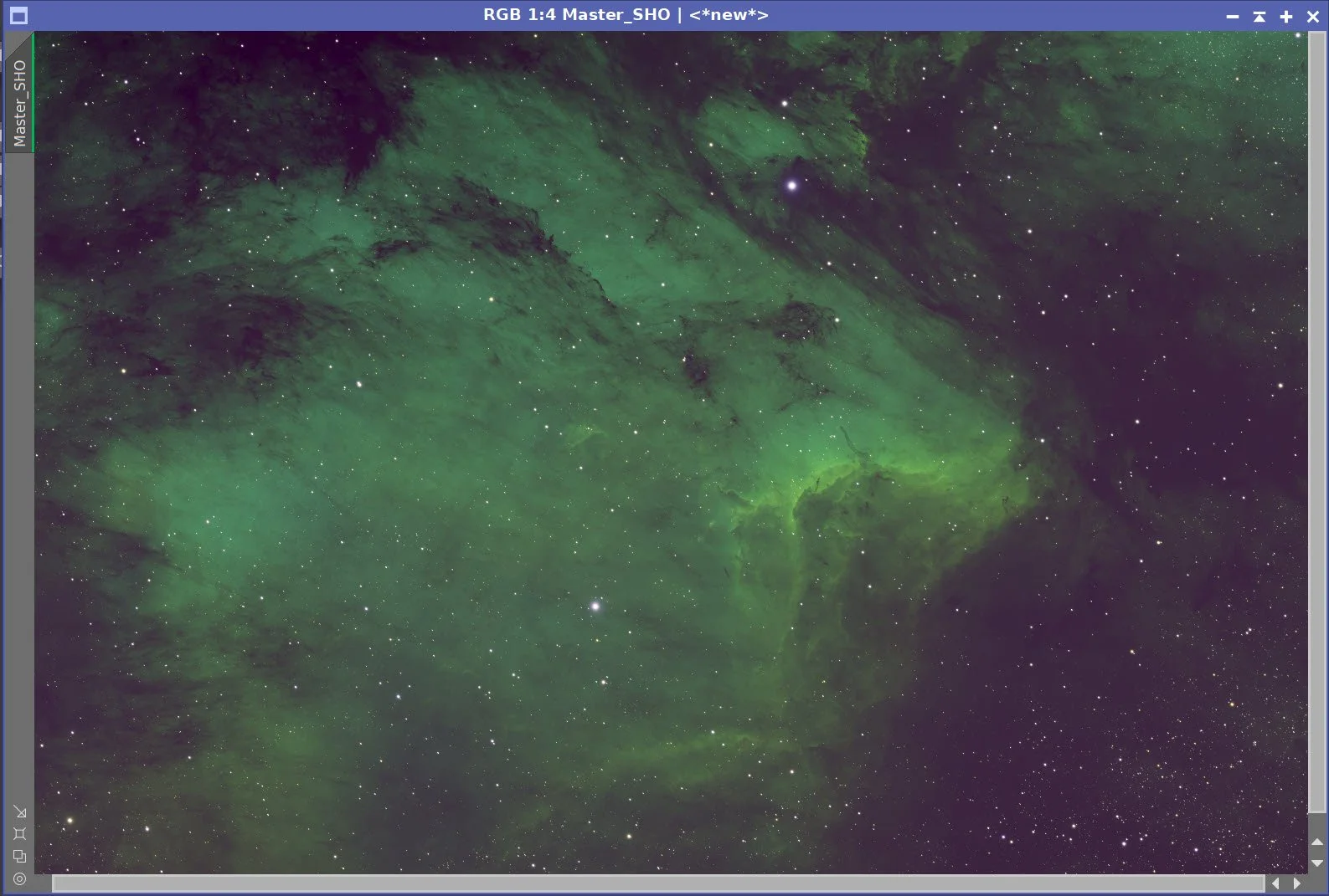
The initial SHO Color image

Measuring Star Sizes.

BXT Paramaters used.

NXT Parameters used.
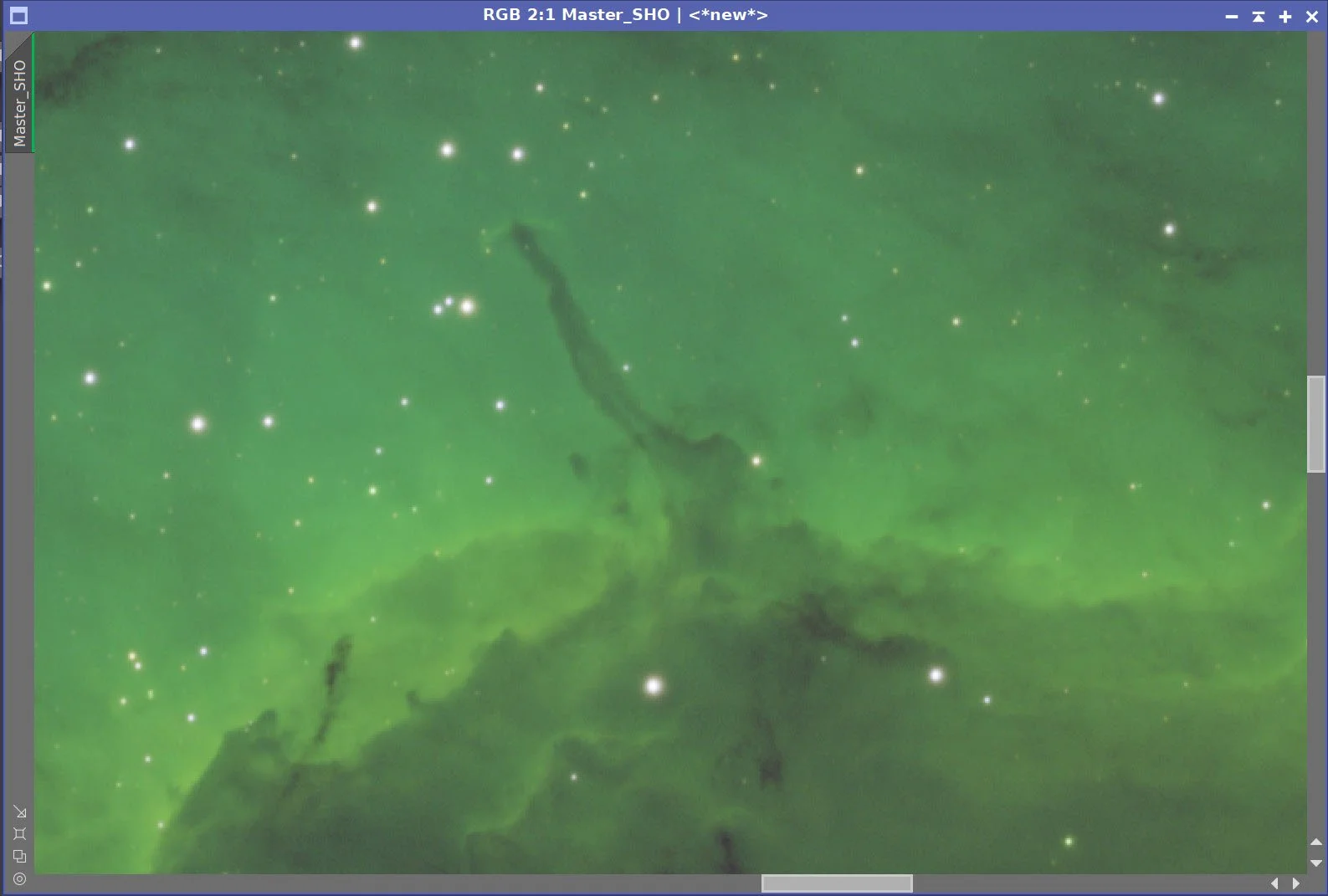
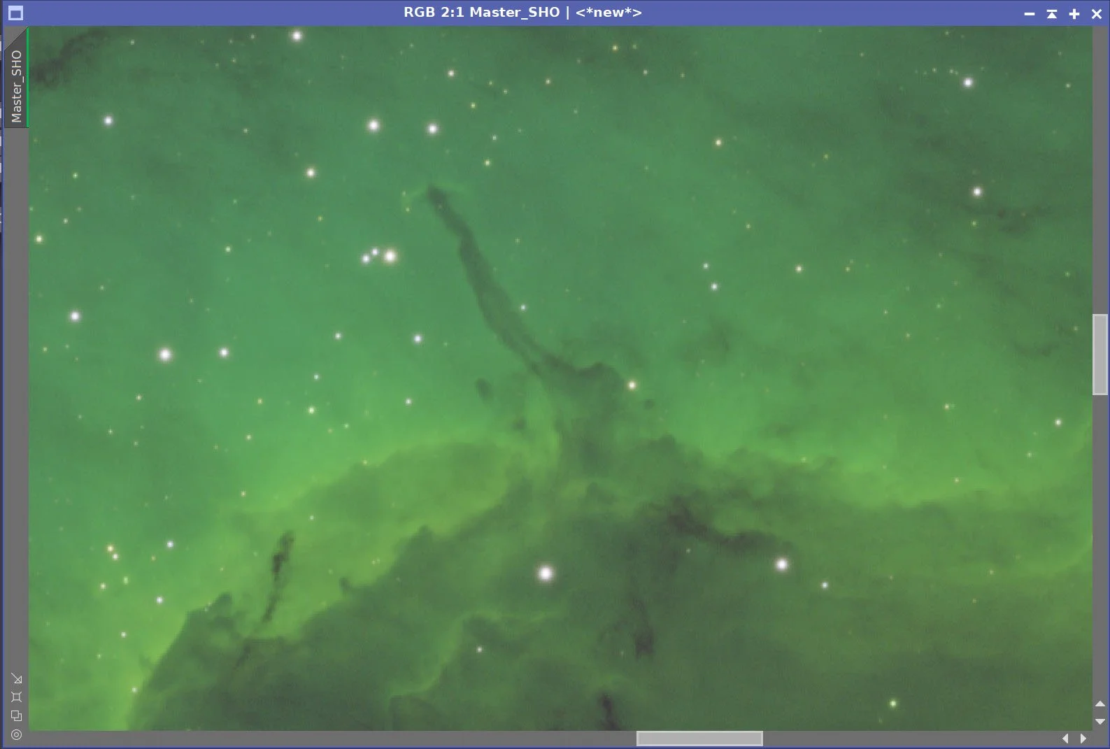


The Master SHO Image before BXT, After BXT Correction only, After BXT Full Correction, and After NXT V3
The full image after the BXT sequence.
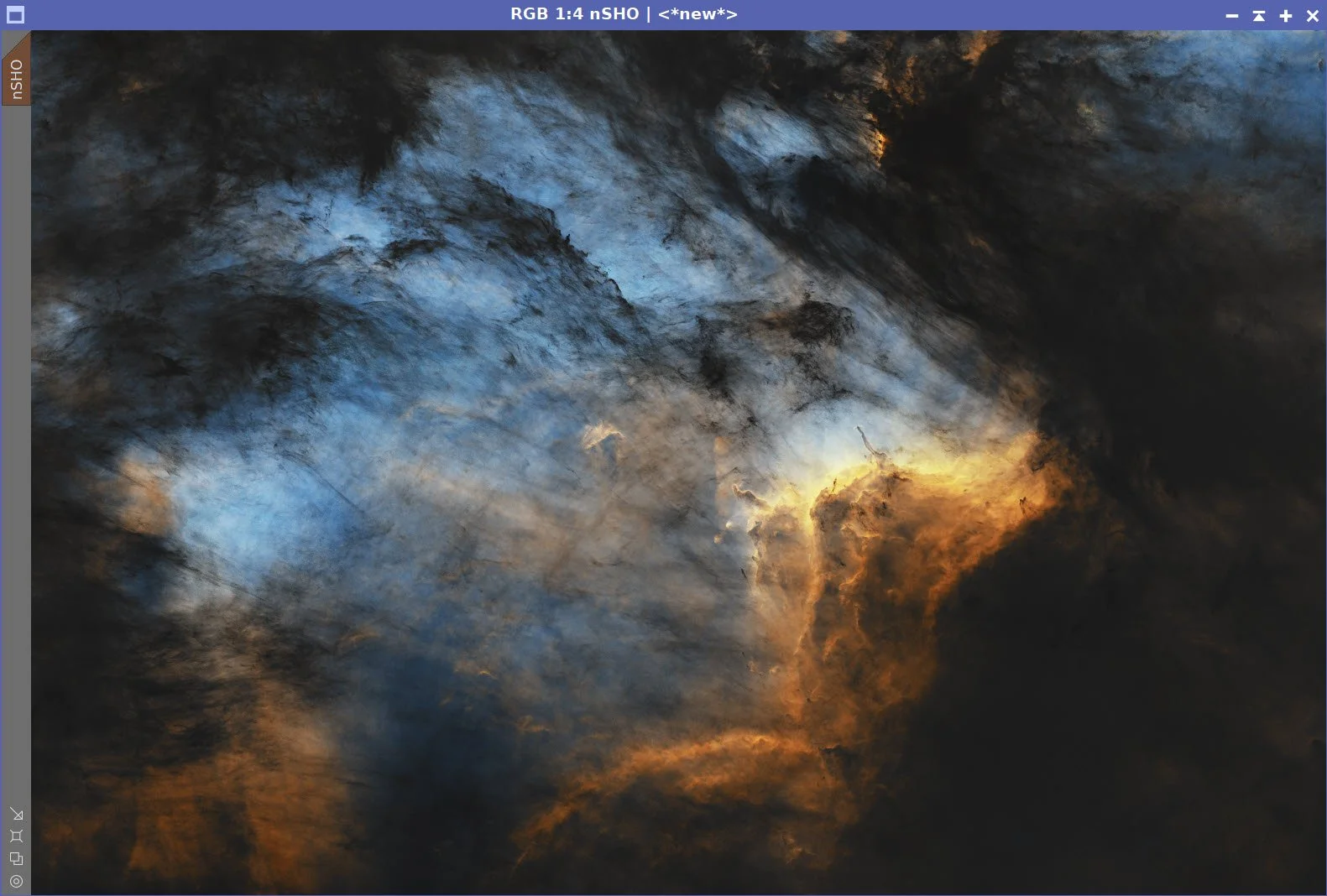
After running SXT: SHO Starless Image (click to enlarge)
SHO Stars Image resulting from STX. (click to enlarge)
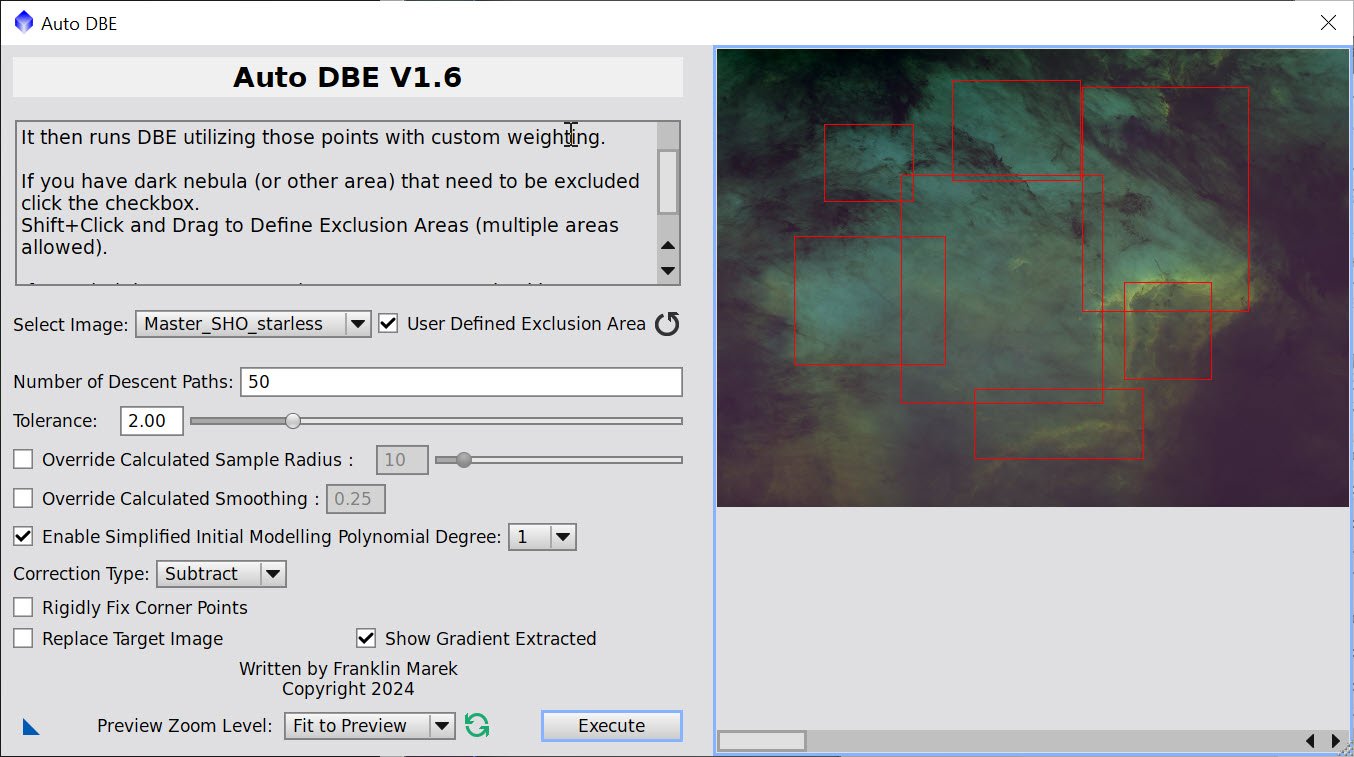
Auto DBE Screen and params used. See the exclusion zones.

NorrowbandNormalization Paramters used.
After NarrowbandNormalization
5. Take the Star and Starless Image Nonlinear
For both images, use the STF->HT method to go nonlinear. Rather than show the images again, we will pick them up in the next processing sections.
6. Process the Nonlinear SHO Starless Image
Use the Istorgram Tool (HT) to move the black point to the right a bit.
Use CT to adjust tone scale and color saturation.
There is still a lot of magenta in the image. To get rid of it, we will do the following sequence:
Invert the Image (magenta becomes green!)
Run SCNR Green at 100% (remove green)
Invert the image
Do a global CT adjust. (dial things back in now that magenta is gone)
Create Color Masks
Use ColourMask to create a WarmMask with hues from 330 to 72
Use ColourMask to create a CoolMask with hues from 162 to 256
Use ColourMask to create a Yellow Mask with hues from 50 to 76
Apply the WarmMask
Use CT to adjust brightness, saturation, and red content
Use LHE (LHE1: radius 64, max contrast 2.0, Amount 0.4, 8-bit histogram) to enhance small-scale detail.
Use LHE ( LHE2: radius 230, max constrat 2.0, amount 0.3, 10-bit histogram) to enhance larger-scale detail.
Apply the CoolMask
Use CT to adjust brightness, saturation, and red content
Apply the YellowMask
Use CT to adjust brightness, saturation, and red content
Perform a modest sharpening with MLT - refer to the screenshot for the parameters used.
The initial SHO color image (click to enlarge)
After gloabl CT adjust(click to enlarge)
After SCNR Green 01.0 (click to enlarge)
Use HT to move the blackpoint (click to enlarge)
Inverting the image. The magenta background is now green. (click to enlarge)
After another invert image. Magenta background is gone. (click to enlarge)
After a global CT adjust.

WarmMask Creation
WarmMask (click to enlarge)
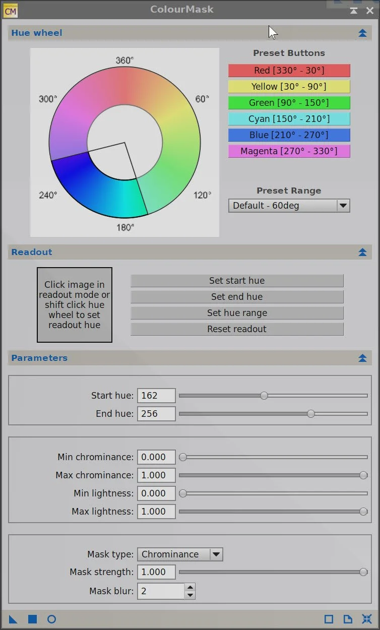
CoolMask Creation.
CoolMask (click to enlarge)
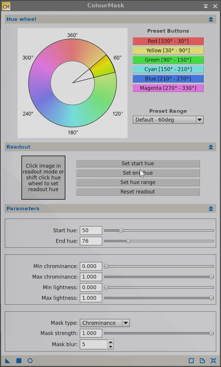
YellowMask Creation
YellowMask (click to enlarge)
Adjust using CT with the WarmMask (click to enlarge)
Adjust with LHE2 and WarmMask (click to enlarge)
Adjust CT with YellowMask (click to enlarge)
Adjust with LHE1 and WarmMask (click to enlarge)
After CT with the CoolMask (click to enlarge)

Sharpening Params used.
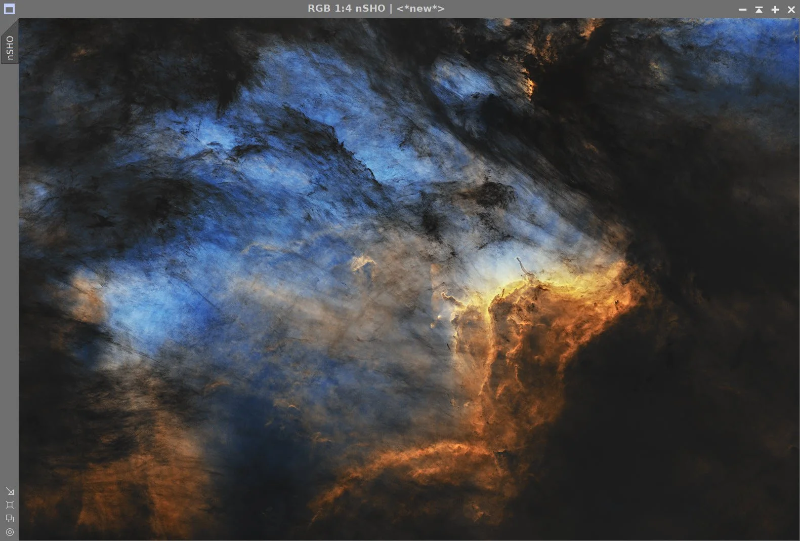
After Sharpening, this is the final starless image.
7. Process the SHO Stars
We start with a nonlinear SHO star image.
I am going to try the Seti Astro NB-to-RGB-Stars Script, which wants separate Ha, O3, and S2 images as input. To get that, I am going to extract the mono images and call them R, G, and B - corresponding to S, H, and O.
I use the script panel and preview to get a look I like - see screen snap below.
Lately, I have needed to increase the star sizes so that they compete with strong areas of nebulosity. Using CT, I will start with my star image and create two more versions with the stars brightened, making them stand out more. I can then use these with the ScreenStars Script to create different versions and see what I like best.
Initial SHO Stars Image (click to enlarge)
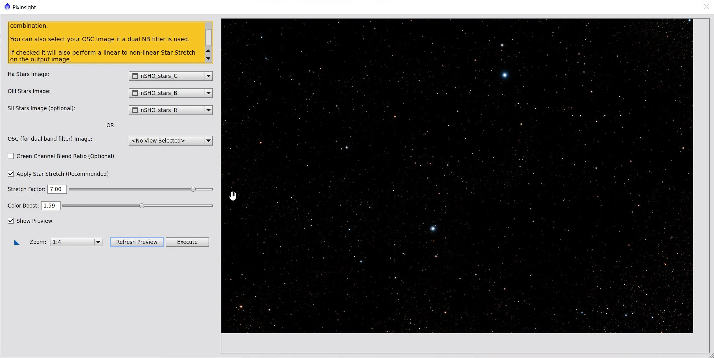
NB-to-RGB-Stars Script. Parameters used.

Three star images - each with progressively more enhanced stars.
9. Add Stars Back In
Use the ScreenStars Script to create three images with the various-sized stars.
Choose the best. I liked the largest best.
Use this script to create three starred versions,
Smallest Stars (click to enlarge)
Middle-sized stars (click to enlarge)
Largest Size stars (click to enlarge)
Final image for polishing.
8. Export the Image to Photoshop for Polishing
Save the image as a TIFF 16-bit unsigned and move to Photoshop
Make tiny global adjustments with Clarify, Curves, and the Color Mixer
Added Watermarks
Export Clear, Watermarked, and Web-sized jpegs.

The Final Image!