
WR 134 - A Wolf-Rayet Star Region In Cygnus- 15.5 Hours in SHO
Date: October 16, 2023
Cosgrove’s Cosmos Catalog ➤#0130
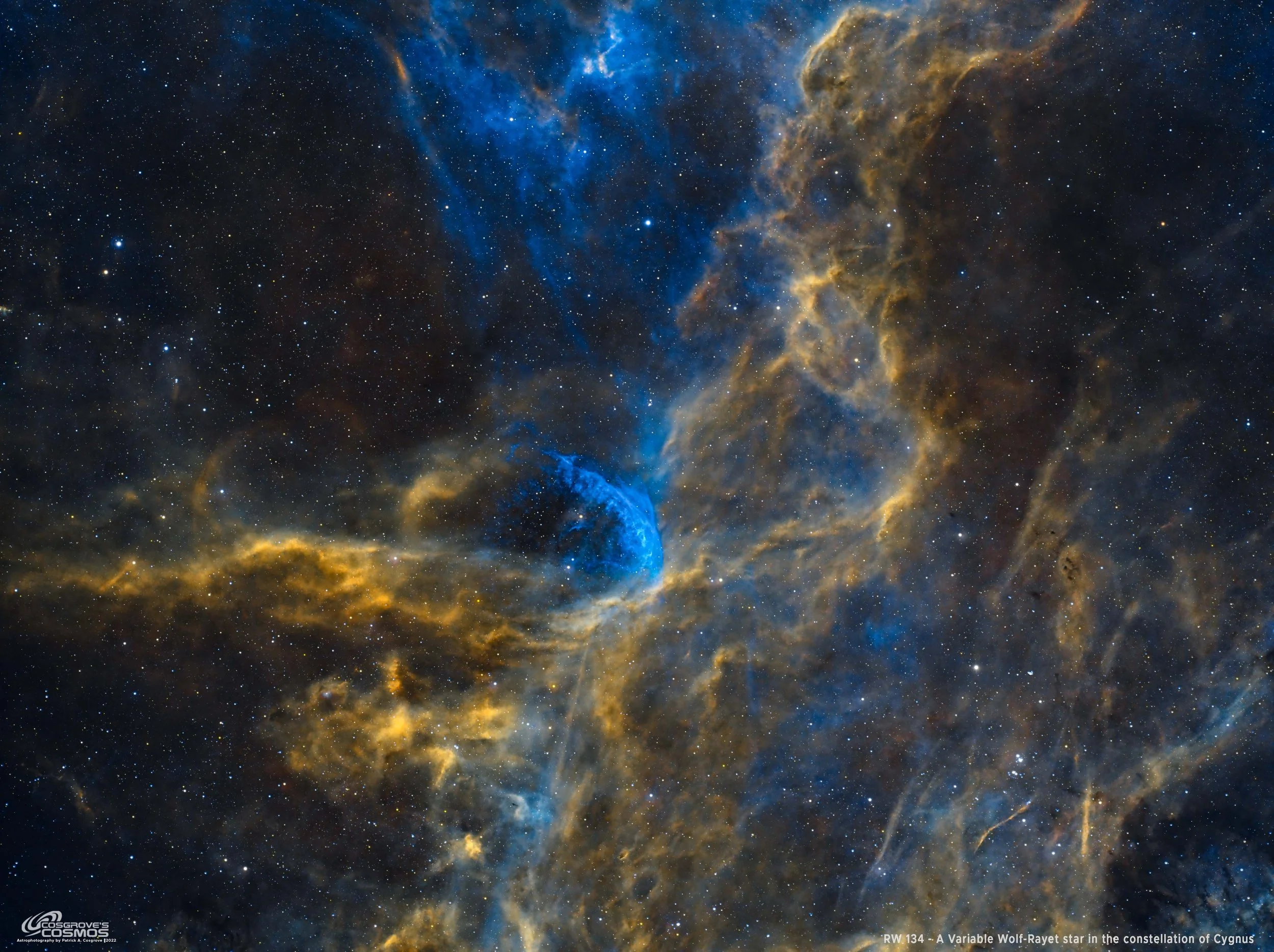
This region in Cygnus is busy and complex! Centered on WR 134 - A Wolf-Rayet Star in a bubble of gas! (click to see the High-Res version via Astrobin.com)
Table of Contents Show (Click on lines to navigate)
Imaging Project #3 From Data Collected During the Recent Clear Weather!
This is the third and final Imaging Project from the recent Data Collection effort in late September. It took me a while to get to it as I was upgrading my main image-processing computer, which took a while.
On the one hand, I am glad to have completed this project.
On the other hand, I fear that this may be my last New image of the year - as the clouds tend to move in and stay around at this time of year. Maybe I will get lucky and have another capture opportunity. I can hope.
But if not, I will end the year with only six new images - which is sad as I have gotten 20 or 30 new images in most years!
About the Target

Spectrum of WR137 showing the emission lines associated with Wolf-Rayet Stars.
WR 134 is a variable Wolf-Rayet star located about 6,000 light-years away in the constellation of Cygnus. This star is bright and massive, having a radius that is five times greater than our own Sun, and has a temperature of 63,000K, making it 400,000 times more luminous!
It is surrounded by a faint bubble nebula formed by this star's intense radiation and solar wind.
This star and two other stars (also shown in this image - see the Annotated image below) were the first three Wolf-Rayet class of stars Discovered. They were observed in 1867 by Charles Wolf and Georges Rayet, using the 40 cm Foucault telescope at the Paris Observatory. These stars displayed board emission lines in their spectrum. Most stars only show absorption lines, making these stars very unusual.

Charles Wolf (1827-1918)

Georges Rayet (1839-1906)
These stars are designed as HD 191765, HD 192103, and HD 192641 - and are also designated in the Wolf-Rayet catalog as WR 134, WR 135, and WR 137, respectively.
The area covered by this image includes a host of other objects. These include NGC 6871, NGC 6883, and other LDN and LBN objects.
So what, exactly, are Wolf-Rayet Stars?
Wolf-Rayet Stars (from Wikipedia)
Wolf–Rayet stars, often abbreviated as WR stars, are a rare heterogeneous set of stars with unusual spectra showing prominent broad emission lines of ionised helium and highly ionised nitrogen or carbon. The spectra indicate very high surface enhancement of heavy elements, depletion of hydrogen, and strong stellar winds. The surface temperatures of known Wolf–Rayet stars range from 20,000 K to around 210,000 K, hotter than almost all other kinds of stars. They were previously called W-type stars, referring to their spectral classification.
Classic (or population I) Wolf–Rayet stars are evolved, massive stars that have completely lost their outer hydrogen and are fusing helium or heavier elements in the core. A subset of the population I WR stars show hydrogen lines in their spectra and are known as WNh stars; they are young, extremely massive stars still fusing hydrogen at the core, with helium and nitrogen exposed at the surface by strong mixing and radiation-driven mass loss. A separate group of stars with WR spectra are the central stars of planetary nebulae (CSPNe), post-asymptotic giant branch stars that were similar to the Sun while on the main sequence but have now ceased fusion and shed their atmospheres to reveal a bare carbon-oxygen core.
All Wolf–Rayet stars are highly luminous objects due to their high temperatures—thousands of times the bolometric luminosity of the Sun (L☉) for the CSPNe, hundreds of thousands L☉ for the population I WR stars, to over a million L☉ for the WNh stars—although not exceptionally bright visually since most of their radiation output is in the ultraviolet.
The naked-eye stars Gamma Velorum and Theta Muscae, as well as one of the most massive known stars, R136a1 in 30 Doradus, are all Wolf–Rayet stars.
The Annotated Image

This annotated image was created using the ImageSolver and AnnotateImage Scripts in PixInsight.
The Location in the Sky

This annotated image created with Imagesolver and Annotate Image Scripts in Pixinsight.
About the Project
Realizing that I would soon have a weather window with the New Moon, I began searching for the targets I wanted to go after.
Cygnus was well placed in the sky, and it holds so many objects that it is naturally a happy hunting ground for astrophotographers.
So, I scanned Astrobin using their “Explore Constellation” feature and found an image of this target. I thought it looked like a fascinating section of sky, and I was intrigued by the prospect of imaging the first three Wolf-Rayet stars ever discovered and even more interested in learning more about this class of objects.
Data Collection
I was fortunate in that my target would be transecting the widest area between my two treelines.
This was the first time I could shoot since I paid a Tree Outfit earlier in the year to come out and widen my tree access window to the sky. As a result, I could get over 5 hours a night for a given target when it is crossing at the widest portion@
This is a record for me for a single target!
The first and second nights were very clear, calm, and cool. I was very confident that I was getting good data. The guiding numbers I saw were some of the best results I have ever seen from this AM5 mount, often coming in as low as 0.24!
After two nights, the clouds came in, and I was shut down.
But the weather was predicted to improve a few days later, and on the 21st, it was expected to be clear for about 2 hours after dark. I thought I would continue to collect narrowband subs until the clouds came in and shut me down.
However - the conditions were better than expected! I shot all night long - getting another 5 hours of data capture.
Data Analysis
I did a blink analysis on all the images, and the data generally looked quite good. I saw some satellite and meteor trails and some slight cloud gradients.
The Ha data showed some frames with these effects but none significant enough to warrant removal.
The O3 data had four removed for cloud issues.
The S2 data tended to be shot towards the end of each night and, because of this, had some frames where the target descended into the water treeline. Four images were removed because of this issue. I also had one frame with some tracking issues, which was also removed.
In total, I removed nine subframes - which means I lost only 45 minutes of integration time. Not great, but not horrible either.
The flats and darks all looked good.
Image Processing
Narrowband Only
This was a narrowband project. For the other projects in this group, I took the time to collect some RGB data so that I could have RGB stars for use in my final image. I did not do that here, and now I kind of wish I had.
I think RGB stars would have been a nice addition to this project. I did not collect RGB star data because I was very concerned that I needed as much integration as I could get to best show the faint aspects of this target. In hindsight, this was probably a bad call.
NarrowbandNormalization Script
Bill Blanshan has created some excellent PixelMath Scripts for Astro Processing, and one of the scripts he made in the past year was focused on NarrowbandNormalization. I have used this script in the past and gotten good results. I have also used it and gotten terrible results. So - to be honest - I was not that much of a fan of this specific capability (I think some of his other tools are wonderful).
Then, he teamed up with Mike Cranfield and created a true PixInsight Process for this capability.

The new NoarrowbandNormalization Tool
As a PixInsight process, it can now provide support for Live Previews - which allows you to adjust parameters and have real-time feedback on how these changes impact the image.
For NarrowbandNormalization, this has been a huge help. Using the tool was intuitive and allowed me to dial in the look I wanted quickly. I expect to use this more routinely in my narrowband work in the future.
The new process created by Bill and Mike can be found here:
https://cosmicphotons.com/scripts/
Processing Workflow
The workflow I used this time was similar to what I used on my previous project. I created my SHO color image in the linear domain and ran BlurXTerminator (BXT) and NoiseXTerminator. Then, I used StarXTerminator to make stars and starless versions.
These were then taken to the nonlinear domain using a simple HistrogramTransformation method.
Once in the linear domain, I used the NarrowbandNormalization tool as the first step in my processing chain in this domain.
After processing the SHO Starless image, I worked on the stars. I used the CurvesTransformation (CT) and the ColorSaturation Tool to try and make the star colors look a bit more natural.
Then the star and the starless images were combined to get to the final result.
Here is the high-level workflow used:

The Workflow used for this project.
Final Results
While I was pleased with the final image, I had two areas of disappointment.
The Missing “Ring”
First - I was hoping to be able to capture and show the “Ring” nebula associated with WR134. While I could detect it in my data, everything I tried to do to enhance and bring it out just made the image look unnatural.
The reason, of course, was that I did not have enough integration to show it well.
I have seen example images with 15 hours of integration that do show the ring. So why are they able to see it and I am not?

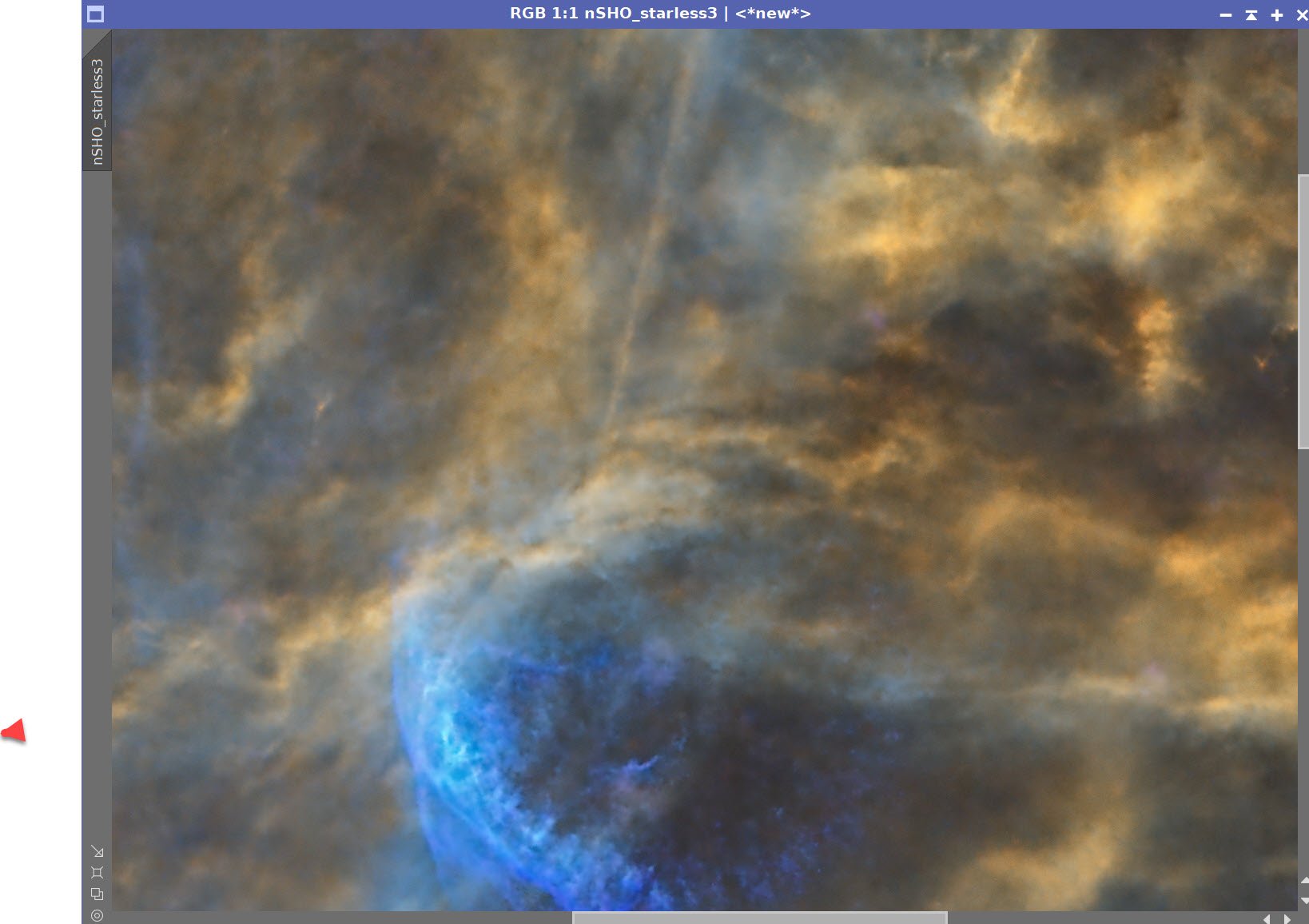
Faint evidence of the “Ring” around WR134 as seen in my O3 Master Starless Image.
Is it because my scope is too slow? I don’t think so - it’s an f/5.5 system, so it’s pretty fast.
Is it because of the filters I am using? Maybe. I am using 6nm Astronomiks. Perhaps if I had a narrower cut in the O3 filter - perhaps 3mm - I might have gotten a cleaner image.
Is it because of the camera I am using? Quite likely! The ASI1600MM-Pro has a peak quantum efficiency of about 60%. If I had been using the ASI2600MM-Pro, that efficiency would have increased to over 90%.
Is it because of where I live? Possibly. We do not have clean, moisture-free skies. If I was imagining from a darker sky site, with a higher elevation to get over some of the atmosphere, or perhaps in a desert climate, I could have possibly done better than I was able to do here in Rochester, NY.
But if you zoom in and look carefully - it is there:

You can see hints of the “Ring” in blue if you look carefully around the edges of the circultar area….
Star Issues
Another concern I had was with the stars. If you zoom in and look at the lower corners of the frame, you will see some stars that have a blue flare shell around them, slightly off-center. Here is an example:

Example of the star problems I was seeing.
Most of the stars don’t show this.
When preparing my “stars” image, I did not notice the problem. I thought the issue appeared once the starless image was combined with the starless image.
However, upon further investigation, I found that the problem was seen in the stars-only image and in the initial linear Master image as well.
I don’t usually see this problem on this scope, and I am still unsure what caused it.
When you look at the image at the normal scale, you don’ really notice it - which is good.
As I shared this with my local group of astrophotographers, they did not seem to think it was a big issue.
Dan Kuchta said, “I know exactly what’s causing this: you’re looking too closely at your image! 😂 “
I guess I can’t argue with that!
The Man/ The Face
One of the folks I shared this image with was Rick Albrecht. While looking at the image, he found that if he looked just so, he could see a “Man” looking back at him. Here is what he saw:

The “Face” in WR134!
Looking at this angle, the bottom of the dark circle looks like a chin, with stars forming the eyes, a nebulous hint of a nose, and a fop of golden hair on top of his head!
This is one of those things where you can't NOT see it once you have it pointed out to you. I think Rick nailed it.
So - Just in time for Holloween - meet the cosmic “Face” in Cygnus!
Look below for the complete step-by-step processing walkthrough! Note: This walkthrough is based upon the use of Pixinsight.
More Information
Wikipedia: WR 134
Wikipedia: WR 135
Wikipedia: WR 137
Wikipedia: Wolf-Rayet Stars
UniverseGuide.com: Facts About WR 134
Nasa APOD for May 18, 2023: An amazing large image scale shot of WR134 showing the “Ring”
ScientificAmerican.com: A great article on Wolf-Rayet Stars that was made known to me by Tony Golumbeck
Capture Details
Lights Frames (after reject removal)
Taken the nights of September 15th, 16th, and 21st, 2023.
66 x 300 seconds, bin 1x1 @ -15C, Gain 100.0, Astronomiks 6nm Ha Filter - 1.25 inch
62 x 300 seconds, bin 1x1 @ -15C, Gain 100.0, Astronomiks 6nm OIII Filter - 1.25 inch
59 x 300 seconds, bin 1x1 @ -15C, Gain 100.0, Astronomiks 6nm SII Filter - 1.25 inch
Total of 15 hours and 35 minutes.
Cal Frames
30 Darks at 300 seconds, bin 1x1, -15C, gain 100
30 Dark Flats at Flat exposure times, bin 1x1, -15C, gain 100
One set of Flats done:
25 Ha Flats
25 OIII Flats
25 SII Flats
Capture Hardware
Scope: Askar FRA400 72mm f/5. 6 Quintuplet Air-Spaced
Astrograph
Focus Motor: ZWO EAF 5V
Guide Scope: William Optics 50mm guide scope
Guide Scope Rings: William Optics 50mm slide-base Clamping Ring Set
Mount: ZWO AM5
Tripod: ZWO TC40 Carbon Fiber tripod w/160mm Extention
Camera: ZWO ASI1600MM-Pro
Camera Rotator: Pegasus Astro Falcon Camera Rotator
Filter Wheel: ZWO EFW 1.2 5x8
Filters: ZWO 1.25” LRGB Gen II, Astronomiks 6nm Ha, OIII,SII
Guide Camera: ZWO ASI290MM-Mini
Dew Strips: Dew-Not Heater strips for Main and Guide Scopes
Power Dist: Pegasus Astro Powerbox Advanced
USB Dist: Pegasus Astro Powerbox Advanced
Polar Alignment
Cam: PoleMaster
Software
Capture Software: PHD2 Guider, Sequence Generator Pro controller
Image Processing: Pixinsight, Photoshop - assisted by Coffee, extensive processing indecision and second-guessing, editor regret and much swearing…..
Click below to visit the Telescope Platform Version used for this image.
Image Processing Walkthrough
(All Processing is done in Pixinsight - with some final touches done in Photoshop)
1. Blink Screening Process
Ha
Some cloud gradients, some trails - no rejects
O3
Some light clouds and some heavy clouds - 4 Rejected
S2
Some gradients
some frames where the target sets into the trees at the end of the night - 4 Rejected
One frame was rejected due to a guide issue
Flats
all fine
Dark Flats
Dark Flats are all fine
2. WBPP 2.5.0
Reset everything
Load all lights
Load all flats
Load all darks
Select - maximum quality
Reg reference - auto - the default
Select the output directory to wbpp folder
Enable CC for all light frames
Pedestal value - auto for all NB filters
Darks -set exposure tolerance to 0
Lights - set exposure tolerance to 0
Lights - all set except for linear defect
Integration - large-scale rejection layer 2x2
set for Autocrop
Set cosmetic corrections for all
No Drizzle
Executed in 46:10

WBPP Calibration View

WBPP Post Calibration View

WBPP Pipeline View
3. Load Master Images
Load all master images and rename them.
Master Ha (click to enlarge)
Master O3 (click to enlarge)
Master S2 (click to enlarge)
4. DBE
No gradients were seen, so I elected to skip DBE
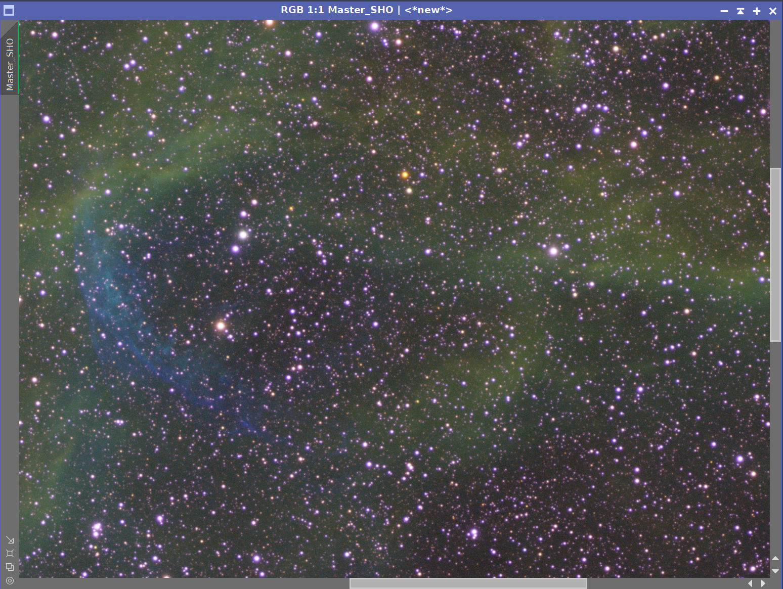
5. Create The SHO Color Image and Do linear Processing
Master SHO (click to enlarge)
Run PSFImage to determine star sizes: X = 1.63 Y = 1.58
I will be using the smaller value - because I assume that we will have any aberrations causing eccentricity removed in the correct first aspect of the BXT run
Run Deconvolution
Experiment with different values
Run BXT - see panel snap for details
Run Noise Reduction
Run NXT with a value of 0.45 - just taking the “fizz off!”

The Output from PSFImage for the Master Ha image.
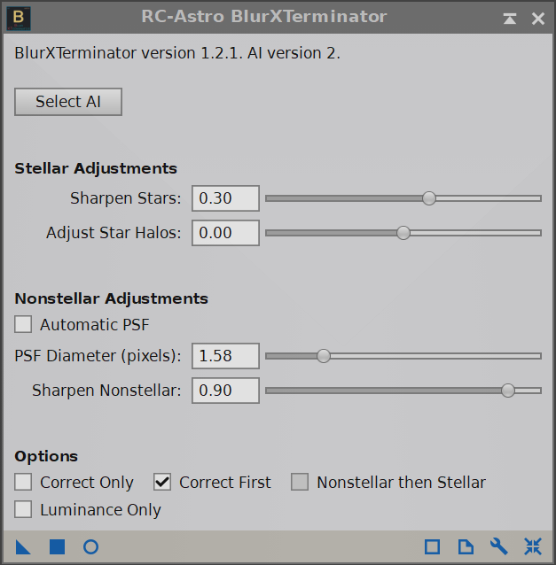
How the BXT tool was configured for the Master Ha image

The Master Ha Image before BXT, After BXT, and After NXT=0.45
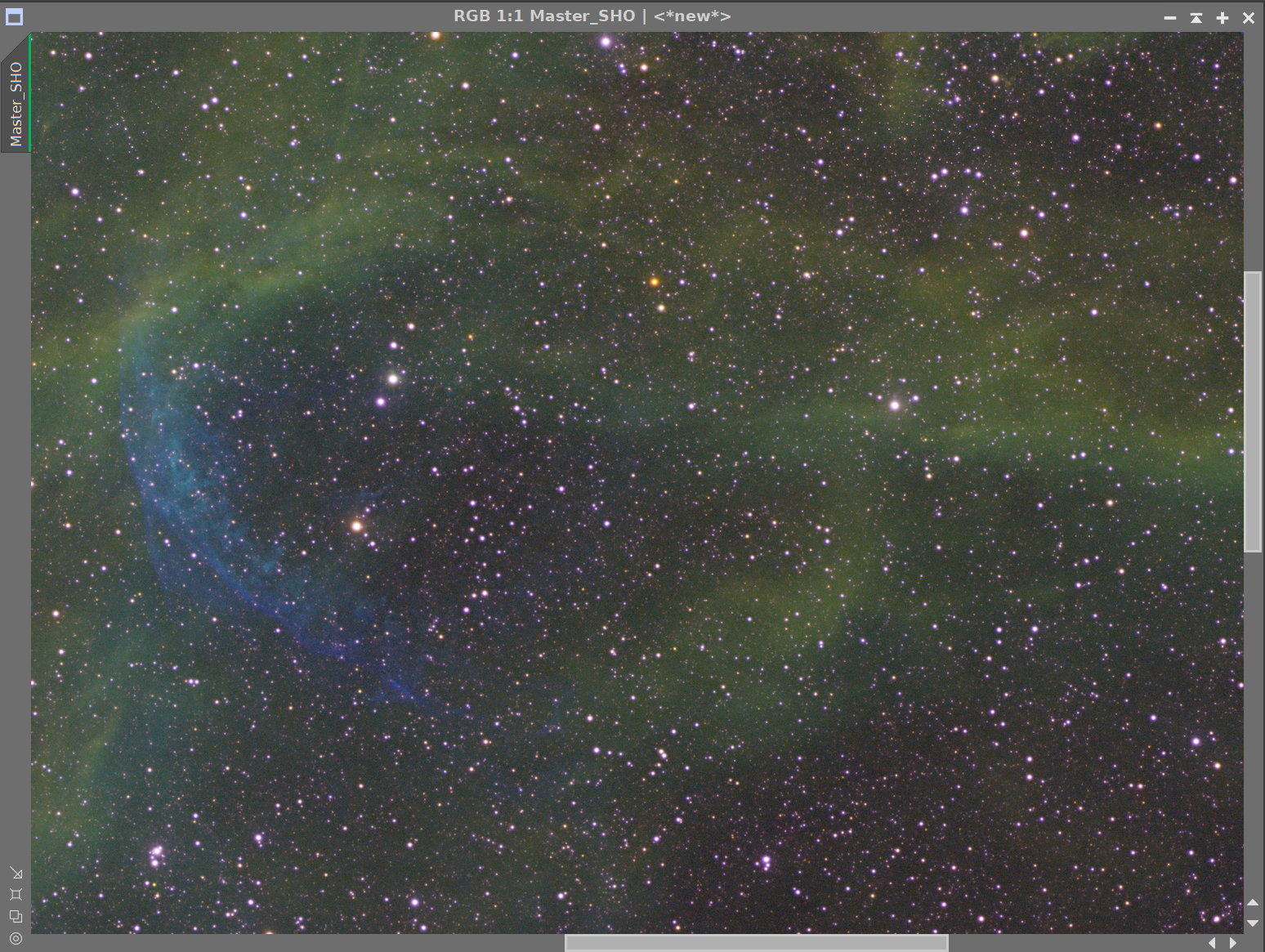
6. Create Starless/Stars-Only Images
Go starless and preserve the star image.
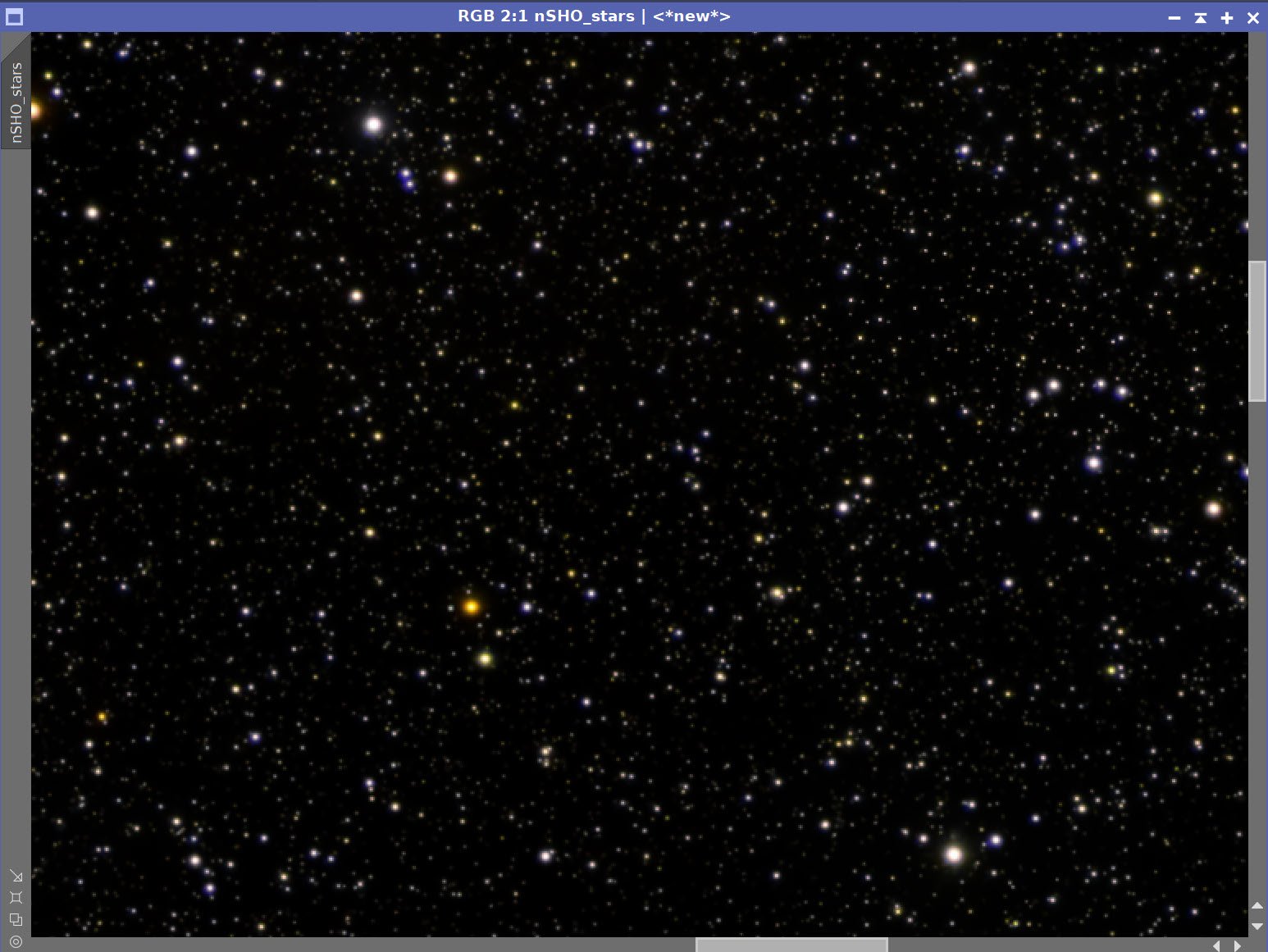
Final Master SHO Image (click to enlarge)
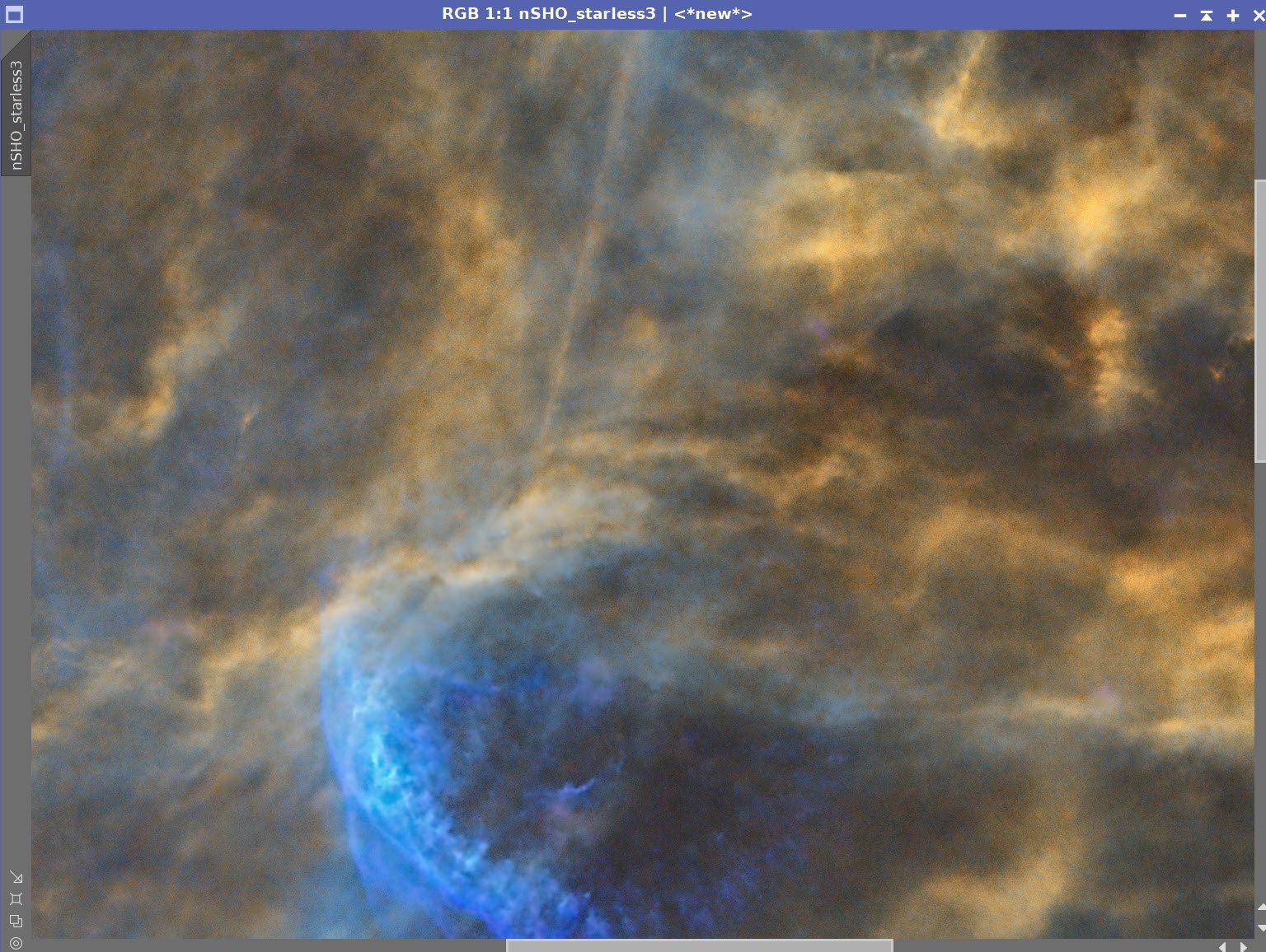
Master SHO Starless Image (click to enlarge)
Final Master SHO Stars Image (click to enlarge)
7. Take SHO Stars Nonlinear and Process
Use HT to bring the stars just to the point where they look good in the nonlinear domain.
Adjust the stars with CT to reduce stars a bit and to enhance their natural color saturation.
Adjust with ColorSaturation to try and make the color stars more normal appearing

SHO Stars after going nonlinear

After CT adjust.

After ColorSaturation Adjust

CT panel setting for star adjustment

The ColorSatuation Panel settings for star adjustment
This is all hard to see, so here is the same series with a zoomed-in portion of the image.

Initial Nonlinear Stars image - zoomed-in

After CT adjust
After ColorSaturation Adjust
8. Take the SHO Starless Image Nonlinear and Process It
Use the STF (unlinked)->HT method to go starless.
Run the Blanshan NarrowbandNormalization Process (see screen snap of panel below)
Create the CoolTonesMask
We will use this to enhance the blueish regions of the image for saturation and detail.
Run ColorMask_Mod with Hue Vectors 172 to 268 (see panel shot below)
Run CT to boost contrast and the mask areas
Run Bill Blanshans’s Mask Blur Tool two times to smooth things out
Apply the Mask and Run CT to adjust the color and tone scale
Create the WarmTonesMask
We will use this to enhance the blueish regions of the image for saturation and detail.
Run ColorMask_Mod with Hue Vectors 332xto 56 (see panel shot below)
Run CT to boost contrast and the mask areas
Run Bill Blanshans’s Mask Blur Tool one time to smooth things out
Apply mask and Run CT to adjust color and tone scale
Apply CoolTonesMask
Run LocalHistogramEqualization (LHE) with radius = 32, contrast limit - 2.0, Amount = 0.25, and an 8-bit histogram
Apply WarTonesMask
Now, we use LHE to enhance detail contrast
Run LocalHistogramEqualization (LHE) with radius = 252, contrast limit - 2.0, Amount = 0.5, and an 10-bit histogram
Run LocalHistogramEqualization (LHE) with radius = 62, contrast limit - 2.0, Amount = 0.5, and an 8-bit histogram
Create the CircleMask using the GAME Script
Create the O2Mask
I hope to use this to enhance the faint “Ring” detail.
Extract the O3 image from the SHO image
Apply CT to boost the contrast
Appy the CircleMask, set to the inverse - use CT to darken the surround to black so you have just the ring portion of the nebula.
Soften lightly with convolution.
Apply the O3Mask
Apply CT
Run NXT = 0. 67
Run UnsharpMask with StdDev = 2.0, Amount = 0.6 to lightness
Apply the CicleMask and adjust CT
The Initial SHO Nonlinear Image (click to enlarge)
After NarrowbandNormalization Process (click to enlarge)
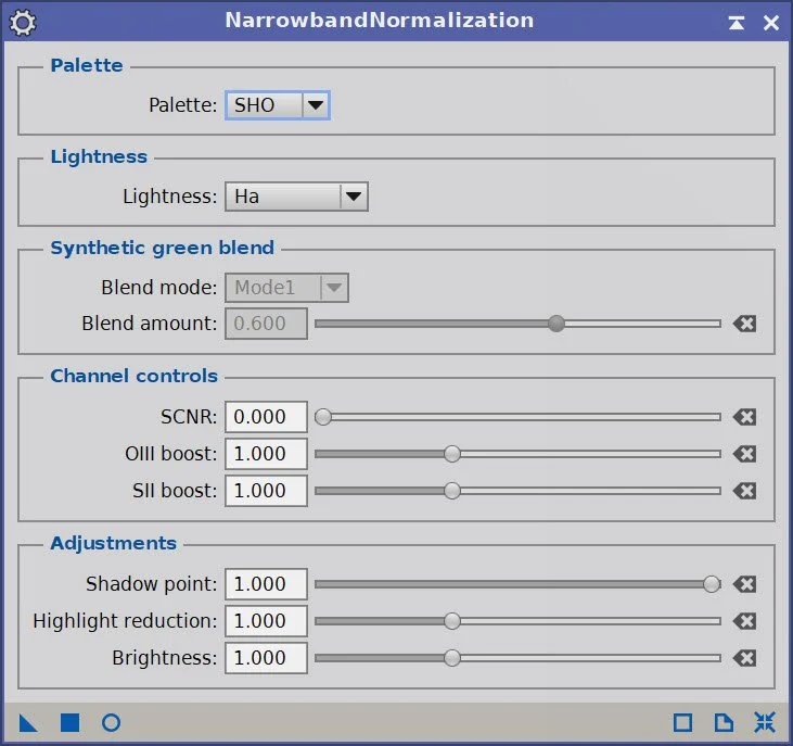
NarrowbandNormalization Panel settings used

After global CT Adjust (click to enlarge)
Creating the CoolTonesMask
The ColorMask_Mod Script Panel Used (click to enlarge)
The Initial CoolTonesMask (click to enlarge)
After a contrast boost done with CT (click to enlarge)
After running the Bill Blanshan Mask Blur tool two times (click to enlarge)
After CT adjust with the CoolTonesMask (click to enlarge)
Creating the WarmTonesMask
The ColorMask_Mod Script Panel Used (click to enlarge)
The initial WarmTonesMask (click to enlarge)
After a contrast boost with CT (click to enlarge)
After smoothing with the Bill Blanshan Mask Blur Tool (click to enlarge)
Apply CT with the WarmTonesMask (click to enlarge)
Apply the WarmTonesMask and run LHE for mid scale enhancement(click to enlarge)
Add the MagentaMask back in and to another CT tweak (click to enlarge)
Apply LHE with CoolTonesMask (click to enlarge)
Apply the WarmTonesMask and run LHE for small scale enhancement(click to enlarge)
Create the CircleMask using the GAME Script

Create the O3Mask
Extract the O3 image from the SHO image (click to enlarge)
Contrast Boost with CT (click to enlarge)
Use CT with the CircleMask Applied to blacken the surround (click to enlarge)
After softening with Convolution (click to enlarge)
Apply CT with O3Mask (click to enlarge)

Before After NXT, and After Unsharp Mask

Apply the CircleMask and Adjust CT
9. Add the Stars Back In and Finish Processing
Use the script ScreenStars to add SHO_Starless and the Stars Images back together
The Final SHO Stars Image (click to enlarge)
The Final SHO Starless Image (click to enlarge)

Combined Image!
12. Export the Image to Photoshop for Polishing
Save the image as Tiff 16-bit unsigned and move to Photoshop
Determine the best image orientation and set
Make final global adjustments with Clarify, Curves, and the Color Mixer
Using the select tool with a feather of 100 pixels, select some feature areas and use clarity to tweak
Add watermarks
Export Clear, Watermarked, and Web-sized jpegs.
Create another version of the image focusing on the Face

The Final Version!

The “Face” version of the image
During August and September I was out shooting every clear night. I had learned a lot of things but I was also noticing several issues that were causing me problems as I did more imaging. I decided to do something to address those issues….