
NGC 6914 - The Spider Nebula (my name!) - 14.5 Hours in SHOrgb
Date: October 6, 2023
Cosgrove’s Cosmos Catalog ➤#0129

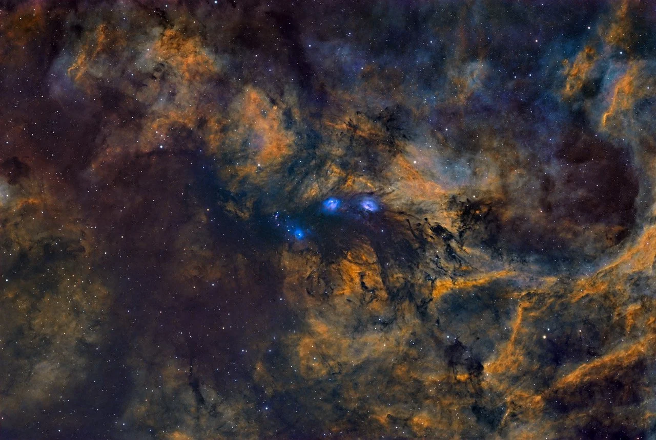
NGC 6914 has no common name that I could find, so I propose calling it the “Spider Nebula!” What do you think? (click to see the High-Res version via Astrobin.com)
Table of Contents Show (Click on lines to navigate)
Imaging Project #2 From Data Collected During the Recent Clear Weather!
After a long year with no nights that were clear of clouds and smoke, I recently had three nights of clear, wonderful skies and could collect data for three projects. The first was SH2-112 - which I recently posted. This is the second in that series.
About the Target
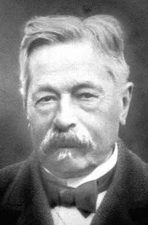
Édouard Jean-Marie Stephan (1837 – 1923)
When it comes to rich areas of the night sky, Cygnus is one of my favorites. With the Milky Way running through this sector of the sky, it is filled with targets that are both well known and some that are not well known - but deserve more attention.
Here is another example of a Target that could use more attention!
NGC 6914 is an Emission and Reflection Nebula located 6,000 light-years away. Ultraviolet light from young hot stars in the Cygnus OB2 Association (home to some of the most massive and luminous stars known) are responsible for ionizing the gas clouds found here, causing them to glow. Also evident are dark dust features that blot out the bright nebulae behind them.
Édouard Stephan discovered this object on August 29, 1881. Stephans was a French astronomer and the director of the Marseille Observatory from 1864 to 1907. He was known for systematically studying nebulae, precisely recording their positions, and discovering many new ones. He is also known for discovering Stephan's Quintet.
The Annotated Image

Annotated version of NGC 6914 created with Pixinsight ImageSolve and AnnotateImage scripts.
The Location in the Sky

This annotated image created with Imagesolver and Annotate Image Scripts in Pixinsight.
About the Project
Realizing that I would soon have a weather window with the New Moon, I began searching for the targets I wanted to go after.
Cygnus was well placed in the sky, and it holds so many objects that it is naturally a happy hunting ground for astrophotographers.
I have shot many targets there - most of which are well-known. After you have a few years of Astro Imaging under your belt, you sometimes revisit things you have shot in the past to see if you can “do it better.” I have done much of this and did not want to do it again. So, I was searching for something unfamiliar or something I felt I could try to do differently.
So, I scanned Astrobin using their “Explore Constellation” feature and found an image of this target. It’s not that this object is not well known - there are a lot of images of it around. It’s just that:
It’s in the NGC catalog, but not many others
It has no common or popular name associated with it
There is not a lot of information available for this target.
The other thing that struck me was that almost all of the images I saw of it seemed to be taken with broadband RGB colors. They all had distinctive red-colored nebulosity showing the Hydrogen II regions.

Doing a search for NGC 6914 on Astrobin - note the “sea of red images!”

Here is a NASA APOD Example of a RGB Broadband image of NGC 6914. Note the dominant reds of the hydrogen clouds. In this image, our friendly little spider appears upside down!
I thought this region of the sky looked pretty interesting, and I thought I might try it in Narrowband rather than broadband RGB. This is a relatively wide field setup, so I thought it would be ideal for my WIlliam Optics 132mm FLT Telescope Platform.
I recently updated this platform with the next-generation ZWO ASI2600MM-Pro camera and a Field flattener/0.8X Reducer that took the scope from an f/7 down to an f/5.5, which also widened the coverage field.
So I had my target, chose which scope I would use, and decided to go narrowband!
A Name?
As I mentioned, this object has no common or popular name.
But every time I see it, I see a funny-looking little spider-like character right in the center of the field.
Because of this, I propose that this object be named “The Spider Nebula!”

Here is our little Spider character!
If you ask me - this is a brilliant idea!
And I know that once you consider this and think about it for a moment, you too will see this as a brilliant idea!
So I encourage you to write your congressman, senator, or member of parliament! Call your president or prime minister! Demand that this popular name be associated with this humble object!
Or, maybe if we just start using this name informally - it just might begin to stick…. You never know!
Data Collection
I was fortunate in that my target would be transecting the widest area between my two treelines.
This was also the first time I have been able to shoot since I paid a Tree Outfit to come and widen my tree access window to the sky. As a result, I could get over 5 hours a night for a given target when it is crossing at the widest portion.
This is a record for me for a single target!
The first and second nights were very clear, calm, and cool. I was very confident that I was getting good data. The guiding numbers I was seeing were some of the best results I have ever seen from this mount!
After two nights, the clouds came in, and I was shut down.
But the weather was predicted to improve a few days later, and on the 21st, it was predicted to be clear for about 2 hours after dark. I thought I would take the opportunity to capture some RGB star subs, and then I would continue to collect narrowband subs until the clouds came in and shut me down.
However - the conditions were better than expected! I ended up shooting all night long - getting another complete night of data capture.
Data Analysis
I did a blink analysis on all of the images, and the data - in general - was quite good - but it was not quite as good as I saw with my first project from this session. I had some thin clouds coming over the target area, and some of this was bad enough that I had to reject some frames.
The Ha data had seven frames removed due to clouds and more that were impacted, but I kept them anyway.
The O3 data had six removed for cloud issues. I also saw some meteors and some gradients.
The S2 data had nine frames removed!
The Red, Green, and Blue Data all looked pretty good.
In total, I removed 22 subframes - which means I lost almost 2 hours of painfully acquired integration time.
I have to tell you - that really hurts!
Image Processing
Much like my last project, the signal was pretty strong in both the Ha and S2 images, but the O3 was on the weak side.
Synthetic Luminance Image?
Again - I chose to refrain from using a synthetic luminance image, being afraid that this would obscure the O3 signal. Before I made this choice, I did create a synthetic luminance image using ImageIntegration - using all six master images as inputs.
This is the image I came up with - followed by the weights that ImageIntegration came up with:

The Master Synthetic Image

The Weights use by ImageIntegration to create the Synthetic Luminance image.
Note that the L image does NOT show the prominent features of the O3 Master image. In fact, the O3 image weight is less than 2%, the Ha is 100%, and the S2 is 7%.
As I have seen before, the Synthetic Luminance Image approach sometimes does not work out well if one of the main filter channels has a very weak signal. So, I chose not to use the Lum/Color processing approach.
Processing Workflow
So, instead, I created RGB and SHO Master color images in Linear space and then ran BXT on them. Then, I used STX to go starless.
Both images were then stretched to nonlinear space for processing.
This time, I did not extract the Ha, O3 & S2 mono images for processing. Instead, I processed the SHO image directly.
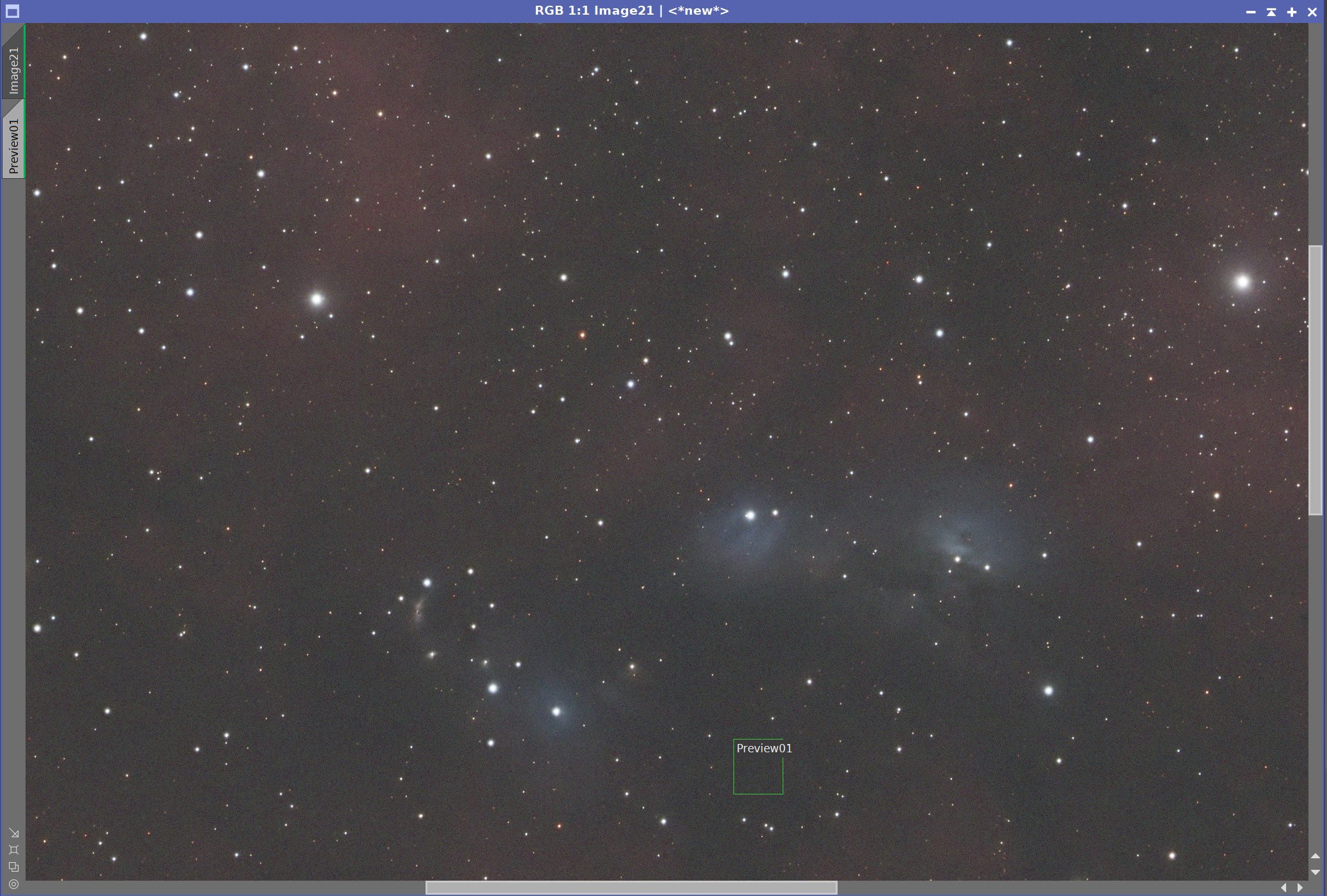
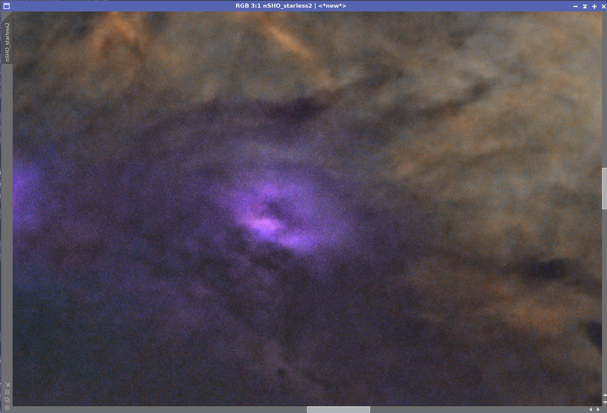
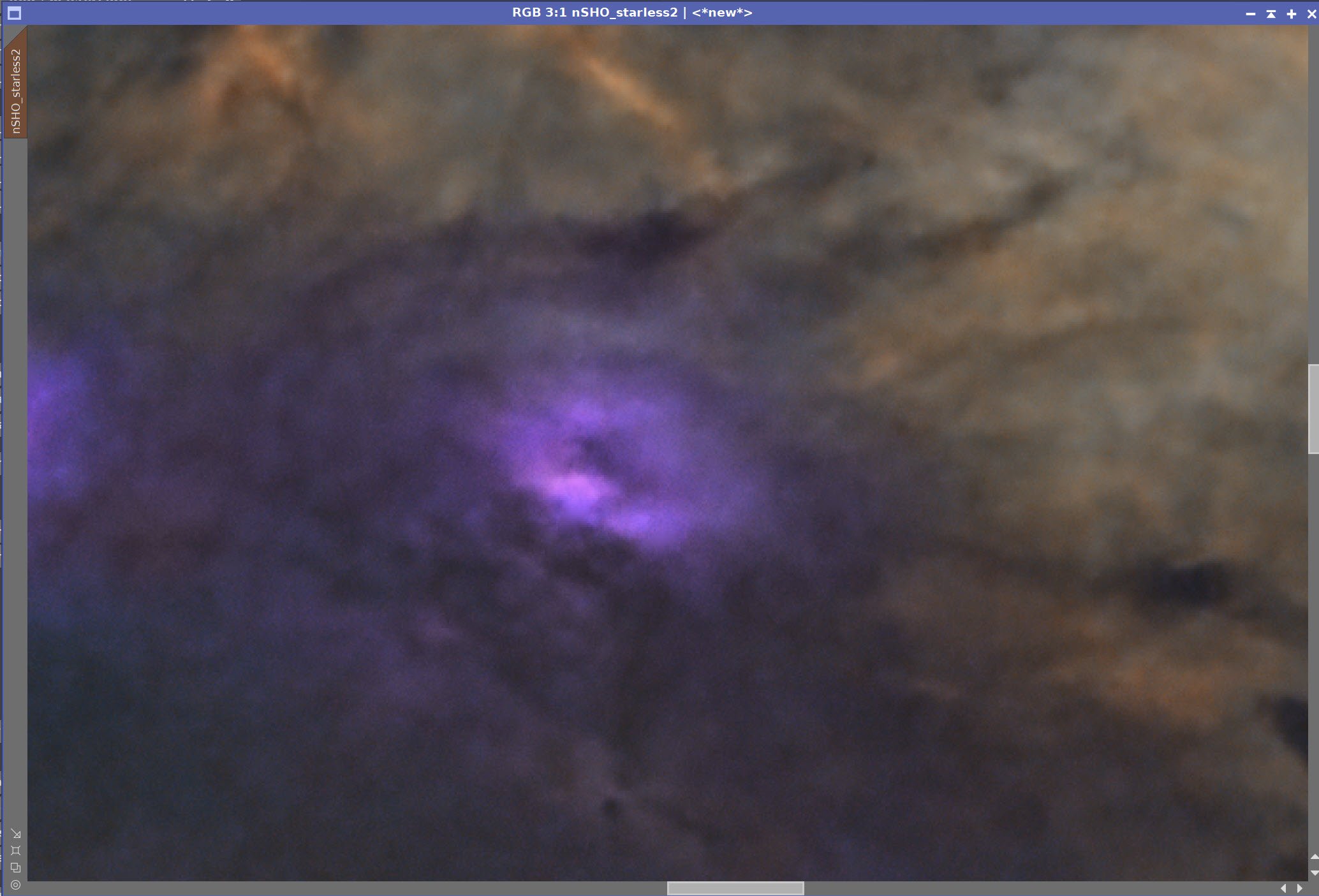
The RGB exposures were very short and taken only to capture natural RGB stars I could use in my final image. However, even at this short integration, I could see some interesting details around the “eyes” of the Spider:
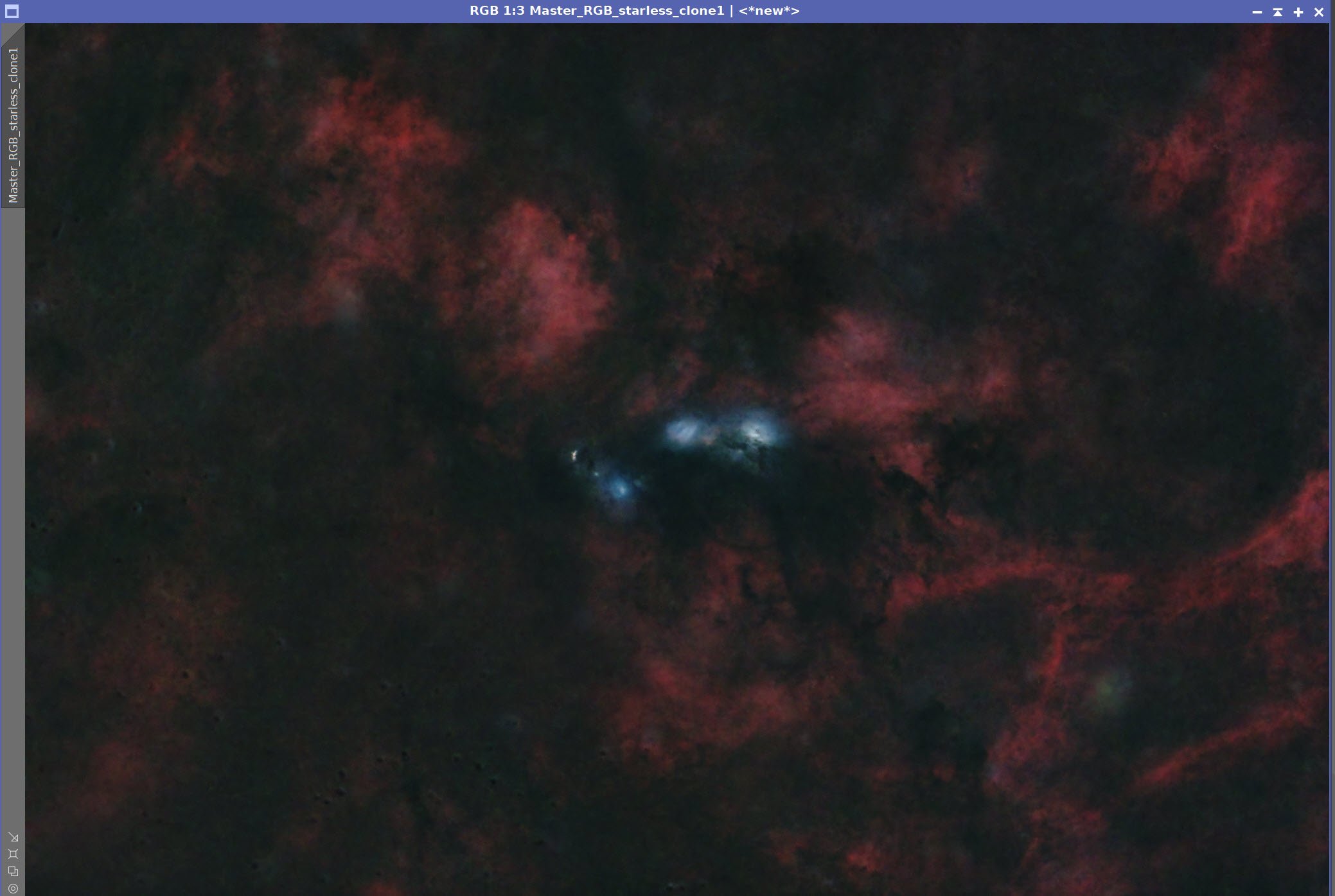
The RGB Starless Image
I decided to take advantage of this, and I created a mask that covered the brightest area of this RGB image, applied that to the SHO image in the later stages of its processing, and folded in a 25 contribution to the final image. This caused the “Eyes” to have even better definition.
This final image was combined with the RGB star image to create the final image.
Here is the high-level workflow used:

The Workflow used for this project.
Feedback
When I finalized the image, I thought that perhaps the image was a bit too green, and I experimented with another color position that was redder and more saturated.
As I often do, I shared with three local colleagues involved in astrophotography. One liked the original best. Another one liked the Redder and stronger color version best. And finally, the third wanted something somewhere between the two!
LOL! Well - that did not solve my problem! But that’s OK - I was asking for opinions, and what I learned from this is that this image was that there was not a simple choice to be made here.
I tried asking for input via X (which - of course - was Twitter. By the way - I think X is a stupid name - not that anyone asked me…):
Hello #Astrophotography Hive Mind!
— 🔭Cosgrove's Cosmos💫 (@CosgrovesCosmos) October 4, 2023
I'm working on an image of NGC 6914 - 14.5 hrs SHO w/rgb stars.
I've two color versions I'm considering. Pick your Favorite!
I'll post the final version with a complete processing walkthrough once I finish the image. pic.twitter.com/ZkozMbfa1A
This did not generate a lot of feedback. This was somewhat surprising as I had gotten a lot of feedback when I had posed a question like this before on that platform. Perhaps the differences between the two positions were not such that people felt compelled to weigh in.
The feedback I did get suggested that this was kind of a split decision. About half liked the original better, and half liked the new one better. There was a slight bias for the original color position, but this was small.
So I hedged my bets - added a bit more saturation to the orange areas of the original image - and called it a day!
Look below for the complete step-by-step processing walkthrough! Note: This walkthrough is based upon the use of Pixinsight.
Capture Details
Lights Frames (after reject removal)
Taken the nights of September 15th, 16th, and 21st, 2023.
55 x 300 seconds, bin 1x1 @ -15C, Gain 100.0, Astronomiks 6nm Ha Filter - 36mm unmounted
59 x 300 seconds, bin 1x1 @ -15C, Gain 100.0, Astronomiks 6nm OIII Filter - 36mm unmounted
57 x 300 seconds, bin 1x1 @ -15C, Gain 100.0, Astronomiks 6nm SII Filter - 36mm unmounted
13 x 30 seconds, bin 1x1 @ -15C, Gain 100.0, ZWO Red Filter - 36mm unmounted
12 x 30 seconds, bin 1x1 @ -15C, Gain 100.0, ZWO Green Filter - 36mm unmounted
12 x 30 seconds, bin 1x1 @ -15C, Gain 100.0, ZWO Blue Filter - 36mm unmounted
Total of 14 hours and 33 minutes.
Cal Frames
30 Darks at 300 seconds, bin 1x1, -15C, gain 100
30 Dark Flats at Flat exposure times, bin 1x1, -15C, gain 100
One set of Flats done:
25 Ha Flats
125 OIII Flats
25 SII Flats
Capture Hardware
Scope: William Optics 132mm f/7 FLT APO Refractor
Flattener/Reducer: P-FLAT7A 0.8X Reducer - new
Focus Motor: Pegasus Astro Focus Cube 2
Cam Rotator: Pegasus Astro Falcon
Guide Scope: Sharpstar 61EDPHII
Guide Focus Motor: ZWO EAF
Mount: Ioptron CEM 60
Tripod: Ioptron Tri-Pier
Camera: ZWO ASI2600MM-Pro
Filter Wheel: ZWO EFW 7x36mm II
Filters: ZWO Gen II 36mm Unmounted LRGB
Astronomiks 36mm Unmounted 6nm Ha, O3, & S2
Guide Camera: ZWO ASI290MM-Mini
Dew Strips: Dew-Not Heater strips for Main and Guide Scopes
Power Dist: Pegasus Astro Pocket Powerbox
USB Dist: Startech 8 slot USB 3.0 Hub
Polar Align Cam: iPolar
Software
Capture Software: PHD2 Guider, Sequence Generator Pro controller
Image Processing: Pixinsight, Photoshop - assisted by Coffee, extensive processing indecision and second-guessing, editor regret and much swearing…..
Click below to visit the Telescope Platform Version used for this image.
Image Processing Walkthrough
(All Processing is done in Pixinsight - with some final touches done in Photoshop)
1. Blink Screening Process
Ha
7 removed for clouds
4 frames were impacted by clouds but kept
O3
Meteors and gradients seen
6 removed for clouds
S2
gradients and clouds seen
9 removed for clouds
Red
Meteor seen, but other than that, the data is clean - no rejections
Green
Clean data - no rejections
Blue
Clean data - no rejections
Flats
all fine
Dark Flats
Dark Flats are all fine
2. WBPP 2.5.0
Reset everything
Load all lights
Load all flats
Load all darks
Select - maximum quality
Reg reference - auto - the default
Select the output directory to wbpp folder
Set the keyword “NIGHT.”
Enable CC for all light frames
Pedestal value - auto for NB filters
Darks -set exposure tolerance to 0
Lights - set exposure tolerance to 0
Lights - all set except for linear defect
Integration - large-scale rejection layer 2x2
set for Autocrop
Set cosmetic corrections for all
Set auto pedestal for narrowband frames
Map flats and darks across nights
Executed in 1 hour ad 34 minutes

WBPP Calibration View

WBPP Post Calibration View

WBPP Pipeline View
3. Load Master Images
Load all master images and rename them.
Master Ha (click to enlarge)
Master Red (click to enlarge)
Master O3 (click to enlarge)
Master Green (click to enlarge)
Master S2 (click to enlarge)
Master Blue (click to enlarge)
4. Create Master Color Images and Run DBE
I will run DBE on the Master Ha, O3, and S2 images and then create the Master SHO image. I am running DBE on the mono images as there appear to be different cloud-driven gradients on some, and I want to clean this up before creating the color SHO image.
For the RGB images, I will create the Master RGB image and then run DEB. I a doing it that way as I do not see any issues with those images, and it is just simpler that way.
DBE was run in subtraction mode.
DBE Sample Pattern for Ha Master (click to enlarge)
Before DBE for Ha Master (click to enlarge)
After DBE for Ha Master (click to enlarge)

Background Pattern - Ha Master (click to enlarge)
DBE Sample Pattern for O3 Master (click to enlarge)
DBE Sample Pattern for S2Master (click to enlarge)
Before DBE for O3 Master (click to enlarge)
Before DBE for S2 Master (click to enlarge)
After DBE for O3 Master (click to enlarge)
After DBE for S2 Master (click to enlarge)
Background Pattern - RGB Master (click to enlarge)
Background Pattern - S2 Master (click to enlarge)
Master SHO (click to enlarge)
Master RGB (click to enlarge)
DBE Sample Pattern for Master RGB image (click to enlarge)
Before DBE for RGB Master (click to enlarge)
After DBE for RGB Master (click to enlarge)
Background Pattern - RGB Master (click to enlarge)
5. Complete the Linear Processing of the RGB Image
Do a Color Calibration
Select a preview sample of the background sky
Setup SPCC panel - see panel snapshot below
Run SPCC
Run Deconvolution
Run BXT - see panel snap for details
Run Noise Reduction
Run NXT with a value of 0.55

Starting RGB image - note the preview sample area - along with the setup of the SPCC panel.

SPCC Output with the regression line.
Master RGB after SPPC (Click to enlarge)

The BXT Panel Setup for the final run
Master RGB Image Before BXT, After BXT, and after NXT = 0.55
6. Do the Linear Processing for the SHO Image
Run PSFImage to determine star sizes: X = 2.177, Y= 1.88
I will be using the smaller value - because I assume that we will have any aberrations causing eccentricity removed in the correct first aspect of the BXT run
Run Deconvolution
Experiment with different values
Run BXT - see panel snap for details
Run Noise Reduction
Run NXT with a value of 0.45
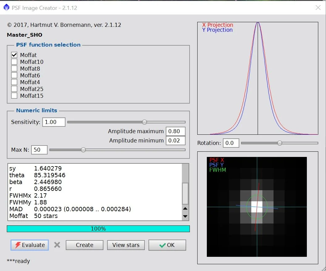
The Output from PSFImage for the Master Ha image.

How the BXT tool was configured for the Master Ha image

The Master Ha Image before BXT, After BXT, and After NXT=0.45
7. Create Starless/Stars-Only Images
For the SHO and RGB images, go starless
Preserve the stars for the RGB
Preserve the starless version for SHO
Final Master SHO Image (click to enlarge)
Master SHO Starless Image (click to enlarge)
Final Master RGB Image (click to enlarge)
Master RGB Starless (click to enlarge)
RGB Star Image (click to enlarge)
8. Take RGB Stars Nonlinear and Process
Use HT to bring the stars just to the point where they look good in the nonlinear domain.
Adjust the stars with CT to reduce stars a bit and to enhance their natural color saturation.

RGB Stars after going nonlinear

After CT adjust.
9. Tale RGB Starless Nonlinear and Process
Use STF->HT method to go nonlinear
Use CT to adjust the tone scale
Appy heavy Noise reduction with NXT = 0.9
The initial RGB Starless Nonlinear Image (click to enlarge)
After CT Adjust (click to enlarge)

The FInal RGB Starless Image After NXT = 0.9 (click to enlarge)
10. Take the SHO Starless Image Nonlinear and Process It
Use the STF (unlinked)->HT method to go starless.
Run SCNR with Green at 0.8
Create a MagentaMask with the ColorMask_mod script
Create the mask with two levels removed
Run CT to boost the contrast
Run Convolution to soften the mask
Apply the MagentaMask and use CT to reduce Magenta tones
Create a WarmTonesMask with the ColorMask_mod script using hue vectors 312-67
Apply CT to boost contrast
Apply Convolution to soften the mask
Apply WarmTones Mask
Run CT to adjust tone scale and sat
Run LHE with Radius 64, Contrast Limit = 2.0, Amount = 0.5, and an 8-bit histogram. This boosts local contrast and detail in the warm tones regions.
Apply another CT to tweak
Apply Global CT
Create the CoolTonesMask using ColorMask_Mod and hue vectors of 160-280
Apply CoolTonesMask
Apply CT to boost contrast
Apply Convolution to soften the mask
Create the SpiderMask
Use GAME to create a gradient mask that covers the spider creature
Apply SpiderMask
Run LHE with Radius 28, Contrast Limit = 2.0, Amount = 0.5, and an 8-bit histogram. This sharpens the edges of the spider.
Run DarkStructureEnhance with default values.
Run NXT = 0.65
I want to enhance the eyes of the spider. They look really good on the RGB_Starless image. So we will add in some of that signal:
Create RangeMask1 - Use RangeSelection on the RGBStarless Image and use the parameters shown in the screenshot below
Apply the mask to the SHO_Starless Image.
Use PixelMath to apply the RGB_Starless image with a 25% weighting function. See the PM Panel shot below.
Do a final CT Tweak.
The Initial SHO Nonlinear Image (click to enlarge)
After SCNR 0.8 on the Green channel. (click to enlarge)
Creating the MagentaMask
The initial MagentaMask from COlrMask_Mod (click to enlarge)
Magenta Mask after CT contrast boost (click to enlarge)
MagentaMask after softening with Convolution (click to enlarge)
After CT adjust with the MagentaMask (click to enlarge)
Creating the WarmTonesMask
The initial WarmTonesMask (click to enlarge)
After a CT contrast boost (click to enlarge)
Smooth with Convolution (click to enlarge)
Apply CT with the WarmTonesMask (click to enlarge)
Final Tweak with CT and WarmTonesMask (click to enlarge)
Add the MagentaMask back in and to another CT tweak (click to enlarge)
Apply LHE with WarmTonesMask (click to enlarge)
After a Global CT Tweak (click to enlarge)
Create the CoolTonesMask
Initial CoolTonesMask (click to enlarge)
Slight contrast Boost with CT (click to enlarge)
Soften the mask with Convolution (click to enlarge)

Apply CT with CoolTonesMask (click to enlarge)
Create the SpiderMask
Make the SpiderMask with GAME (click to enlarge)
SpiderMask Applied (click to enlarge)
After LHE run with the SpiderMask (click to enlarge)
After running the DarkStructureEnhance Script with default params (click to enlarge)
Before and After NXT = 0.65
Create RangeMask_1
RangeMask_1
RangeSlection Parameters used
Before RGB_Starless Contribution (click to enlarge)
After adding in the contribution of RGBStarless using RangeMask1 and PixleMath (click to enlarge)

The Equation used to blend the RGB_starless image in

Do a final CT Tweak (click to enlarge)
11. Add the RGB_Stars Back In and Finish Processing
Use the script ScreenStars to add SHOStarless and the RGB_Stars Image back together
Use Unsharp Mask to sharpen the image a bit - see UnsharpMask panel snap
The RGB Stars Image (click to enlarge)
The SHO_Starless Image (click to enlarge)

Combined Image!

UnsharpMask parameters used.

After sharpening with UnsharpMask
12. Export the Image to Photoshop for Polishing
Save the image as Tiff 16-bit unsigned and move to Photoshop
Adjust with Clarify and Color Mixer
Tweak the color of the spider’s eyes.
Do a final curves.
Add watermarks
Export Clear, Watermarked, and Web-sized jpegs.
Create two versions of the image so I can share and ask for feedback.
One based on the starting color position
Another with a stronger red cast and higher saturation.
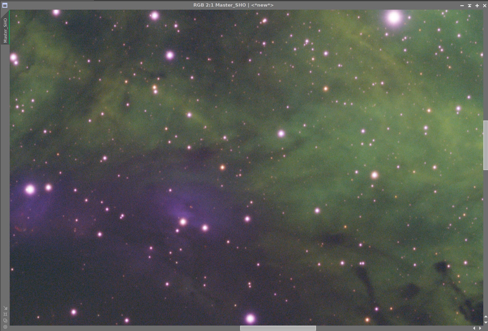
The default color position

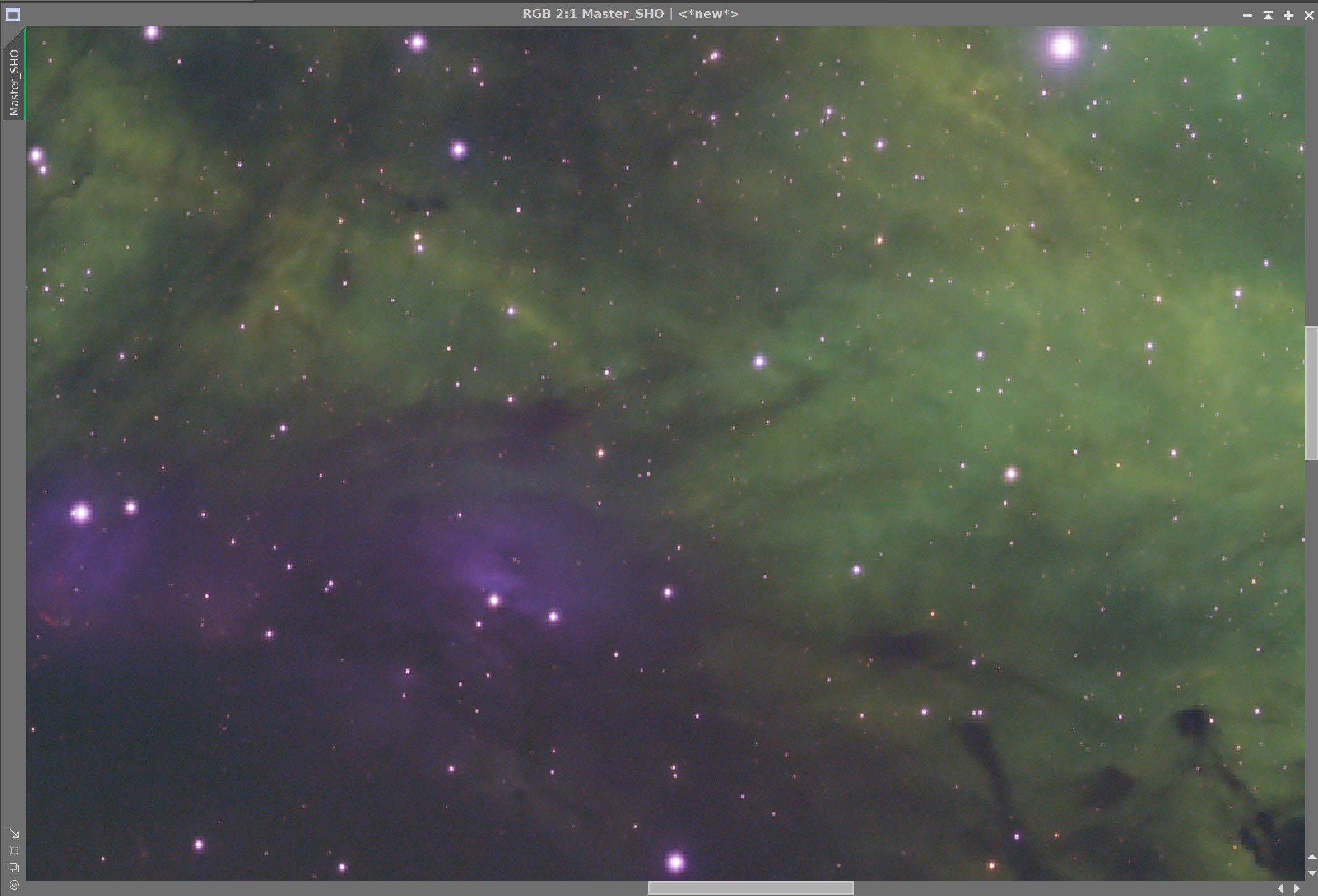
The stronger Red and more saturated version
13. Finalize the Image
I finally created a version that was slightly between the two shown above - by enhancing the color of the gold areas slightly.

The Final Version!
Version 4.0 of the Williams Optics 132mm platform is a major upgrade that involves adding a new 2600 series mono camera, a new 7x36mm EFW and filters, and a new WO Flattener and 0.8X Reducer that will support the larger format sensor and covert the scope to a much faster f/5.5 system.
This post documents the changes and discusses how I planned this change and how it was executed.