
SH2-112 - A Diffuse Emission Nebula in Cygnus - 15.7 Hours in SHOrgb
Date: September 29, 2023
Cosgrove’s Cosmos Catalog ➤#0128

SH2-112 - A beautiful nebula in Cygnus (click image for full resolution via Astrobin.com)
Granted “Explore” Status on Flickr - September 30!

Table of Contents Show (Click on lines to navigate)
Finally! Good Weather and New Data!
2023 has been a terrible year for Astrophotography!
Weather conditions and smoke plumes from the extensive wildfires in Canada have blocked the skies and have greatly limited my ability to capture new data.
I’ve only had three new imaging projects this year thus far. The rest of the time was spent on reprocessing old data. While this has actually been a lot of fun - as I have been able to find better images in that data than I had created before - it is just not the same as jumping in and working with fresh data.
That all just changed!
We had three very clear nights on September 15, 16, and 21! It’s starting to get dark earlier now so I was able to get some good integrations on a number of targets.
This is the first target in that series.
About the Target
SH2-112, also known as LBN 337, is a diffuse emission nebula located about 5,600 light-years away in the constellation of Cygnus. This is a circular region of HII with dark dust rifts that can be seen on the western side. The star responsible for its excitation is believed to be BD+45 3216, a double blue star of spectral class O8V with an apparent magnitude of 9.18.
It is located in a portion of the Orion Spiral Arm that is noted for areas of rich star formation.
Other than that, I have not really been able to find out too much about this object.
It does not seem to have an NGC entry, nor does it have a common name that I could find. While I have found quite a few sample images of this target on Astrobin, it is clearly not one that is well-known in the astro-imaging circles.
The Annotated Image
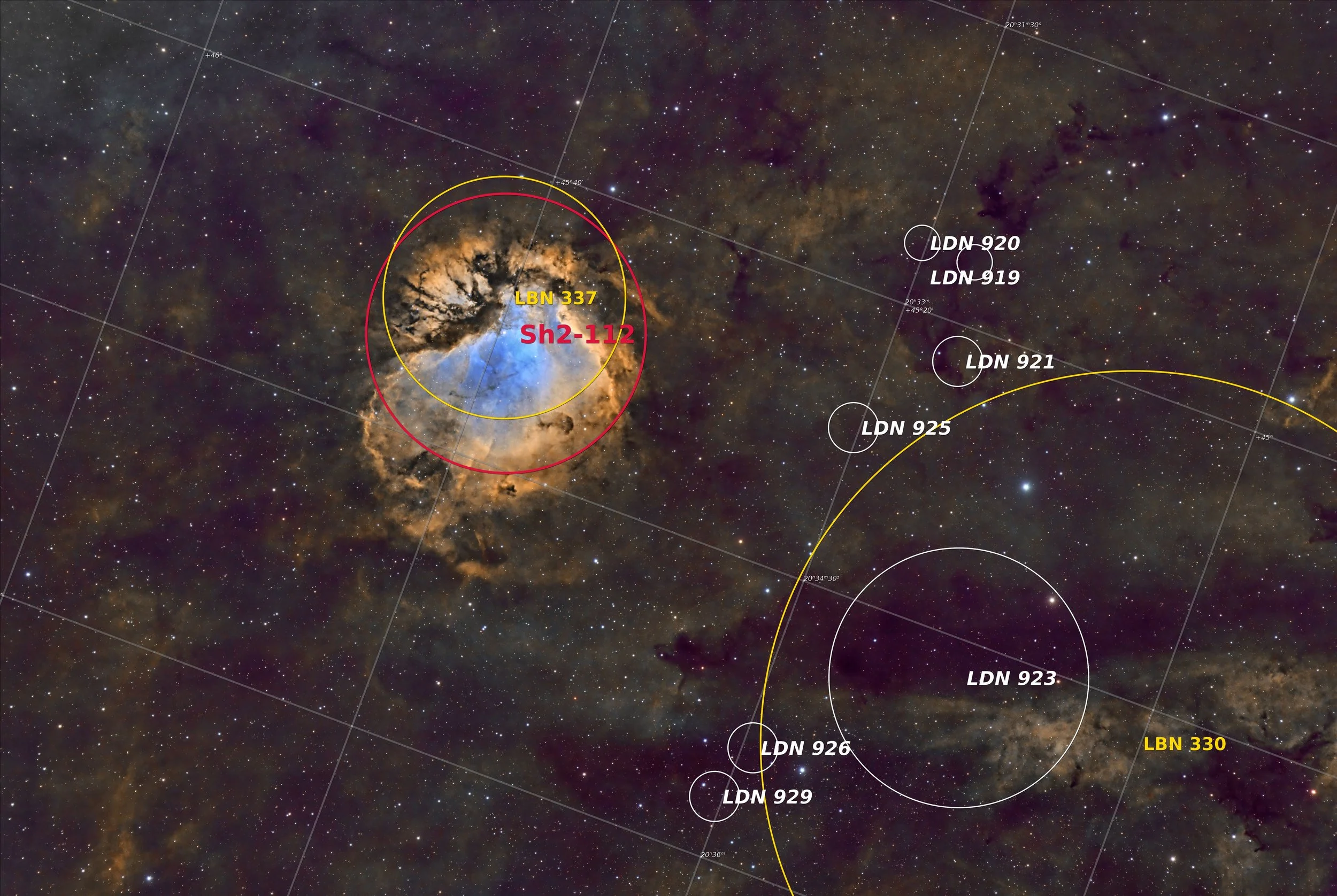
Annotated version of Sh2-112 created with Pixinsight ImageSolve and AnnotateImage scripts.
The Location in the Sky

This annotated image created with Imagesolver and Annotate Image Scripts in Pixinsight.
About the Project
So Finally, we have some clear skies!
As I started looking for targets, I noted that Cygnus was well-positioned. Cygnus is one of my favorite constellations, as it is filled with exciting targets.
So I scanned Astrobin, using their “Explore Contellation” feature and I came across an image of this target. I took note of it because:
It was really neat looking!
I had never heard of it!
I did some searching for more info on it and I found very little. Hmmmm. Even more interesting!
Looking at its size and its detail level, I decided that this would be a good target for my AP130 platform. So I used SGP to create the image composition that I liked and created a sequence for this target.
Data Collection
I was fortunate in that my target would be transecting the widest area between my two treelines.
Also - this is the first time I have been able to shoot since I paid Tree Outfit to come widen my tree window. As a result, I could get over 5 hours a night on the target each night. This is a record for me for a single target.
The first and second nights were very clear, calm, and cool. I was very confident that I was getting good data. The guiding I was getting was some of the best results I have ever seen from this mount!
After two nights, the clouds came in, and I was shut down.
But the weather was predicted to improve a few days later, and on the 21st, it was predicted to be clear for about 2 hours after dark. I thought I would take the opportunity to capture some RGB star subs and then I would continue to collect narrowband subs until the clouds came in and shut me down.
However - the conditions were better than expected! I ended up shooting all night long - getting another complete night of data capture.
Data Analysis
I did a blink analysis on all of the images, and the data - in general - looked quite good.
The Ha data was all clean.
The O3 Data had a handful of frames rejected for light cloud cover. I
n addition - it had two frames rejected because of what looked like frost or dew on the sensor! I have never seen that before.
The S2 data Very slight cloud gradients were seen at times - but nothing too bad.
So - the data looks very promising!
Image Processing
The signal was pretty strong in the Ha and the S2 images, but the O3 was on the weak side.
Typically, I create a synthetic luminance image and use parallel Lum/Color processing paths. However, I have been seeing some cases where this approach hides details in the weaker signal band. So, I opted not to do that this time around.
So, instead, I created RGB and SHO color images in Linear space and then ran BXT on them. Then, I used STX to go starless.
Both images were then stretched to nonlinear space for processing.
The SHO color image had the Ha, O3 & S2 mono images extracted, and then I processed those to maximize the information in each channel. After that, they were recombined into an SHO color image, and then the nonlinear color image was processed and enhanced.
This final image was combined with the RGB star image to create the final image.
Here is the high-level workflow used:
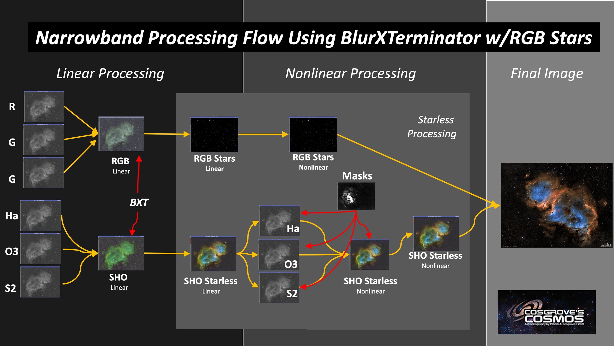
Look below for the complete step-by-step processing walkthrough! Note: This walkthrough is based upon the use of Pixinsight.
More Information
Wikipedia: SH2-112
SharplessCatalog.com: SH2-112
GalaxyMap.com: SH2-112
Space.com: SH2-112
Iopscience.iop.org: Star Formation and Evolution of Blister-type H ii Region Sh2-112 - Thanks to George Killat for finding this one!
Capture Details
Lights Frames
Taken the nights of September 15th, 16th, and 21st, 2023.
68 x 300 seconds, bin 1x1 @ -15C, Gain 100.0, Astronomiks 6nm Ha Filter - 36mm unmounted
61 x 300 seconds, bin 1x1 @ -15C, Gain 100.0, Astronomiks 6nm OIII Filter - 36mm unmounted
53 x 300 seconds, bin 1x1 @ -15C, Gain 100.0, Astronomiks 6nm SII Filter - 36mm unmounted
20 x 30 seconds, bin 1x1 @ -15C, Gain 100.0, ZWO Red Filter - 36mm unmounted
20 x 30 seconds, bin 1x1 @ -15C, Gain 100.0, ZWO Green Filter - 36mm unmounted
20 x 30 seconds, bin 1x1 @ -15C, Gain 100.0, ZWO Blue Filter - 36mm unmounted
Total of 15 hours and 40 minutes.
Cal Frames
30 Darks at 300 seconds, bin 1x1, -15C, gain 100
30 Dark Flats at Flat exposure times, bin 1x1, -15C, gain 100
One set of Flats done:
25 Ha Flats
125 OIII Flats
25 SII Flats
Capture Hardware
Scope: Astro-Physics 130mm F/8.35 Starfire APO built in 2003
Guide Scope: Televue TV76 F/6.3 480mm APO Doublet
Main Fous: Pegasus Astro Focus Cube 2
Guide Fous: Pegasus Astro Focus Cube 2
Mount: IOptron CEM60
Tripod: IOptron Tri-Pier with column extension
Main Camera: ZWO ASI2600MM-Pro
Filter Wheel: ZWO EFW II 7x36
Filters: ZWO 36mm unmounted Gen II LRGB filters
Astronomiks 36mm unmounted 6nm Ha,
OIII, & SII filters
Rotator: Pegasus Astro Falcon Camera Rotator
Guide Camera: ZWO ASI290MM-Mini
Power Dist: Pegasus Astro Pocket Powerbox
USB Dist: Startech 7 slot USB 3.0 Hub
Software
Capture Software: PHD2 Guider, Sequence Generator Pro controller
Image Processing: Pixinsight, Photoshop - assisted by Coffee, extensive processing indecision and second-guessing, editor regret and much swearing…..
Click below to visit the Telescope Platform Version used for this image.
Image Processing Walkthrough
(All Processing is done in Pixinsight - with some final touches done in Photoshop)
1. Blink Screening Process
Ha
Lots of gradients
Few trails
No deletions
O3
A sequence of five frames was deleted due to light cloud cover
Two images were deleted due to what looks like sensor frost! I'm not sure of what happened at the end of night one!
See the example image below.
S2
Some gradients
One meteor fireball was seen!
No deletions
Red
Clean data - no rejections
Green
Clean data - no rejections
Blue
Clean data - no rejections
Flats
all fine
Dark Flats
Dark Flats are all fine

This is an example of one of the two O3 frame rejected due to this dark circle? Sensor Frost?
2. WBPP 2.5.0
Reset everything
Load all lights
Load all flats
Load all darks
Select - maximum quality
Reg reference - auto - the default
Select the output directory to wbpp folder
Set the keyword “NIGHT.”
Enable CC for all light frames
Pedestal value - auto for NB filters
Darks -set exposure tolerance to 0
Lights - set exposure tolerance to 0
Lights - all set except for linear defect
Integration - large-scale rejection layer 2x2
set for Autocrop
Set cosmetic correction for all
Set auto pedastall for narrowband frames
Map flats and darks across nights
Executed in 9 hours ad 43 minutes

WBPP Calibration View

WBPP Post Calibration View

WBPP Pipeline View
3. Load Master Images
Load all master images and rename them.
Create the SHO Master by using ChannelCombination
Create the RGB Master Image by using ChannelCombination
Master Ha (click to enlarge)
Master Red (click to enlarge)
Master O3 (click to enlarge)
Master Green (click to enlarge)
Master S2 (click to enlarge)
Master Blue (click to enlarge)
Master SHO (click to enlarge)
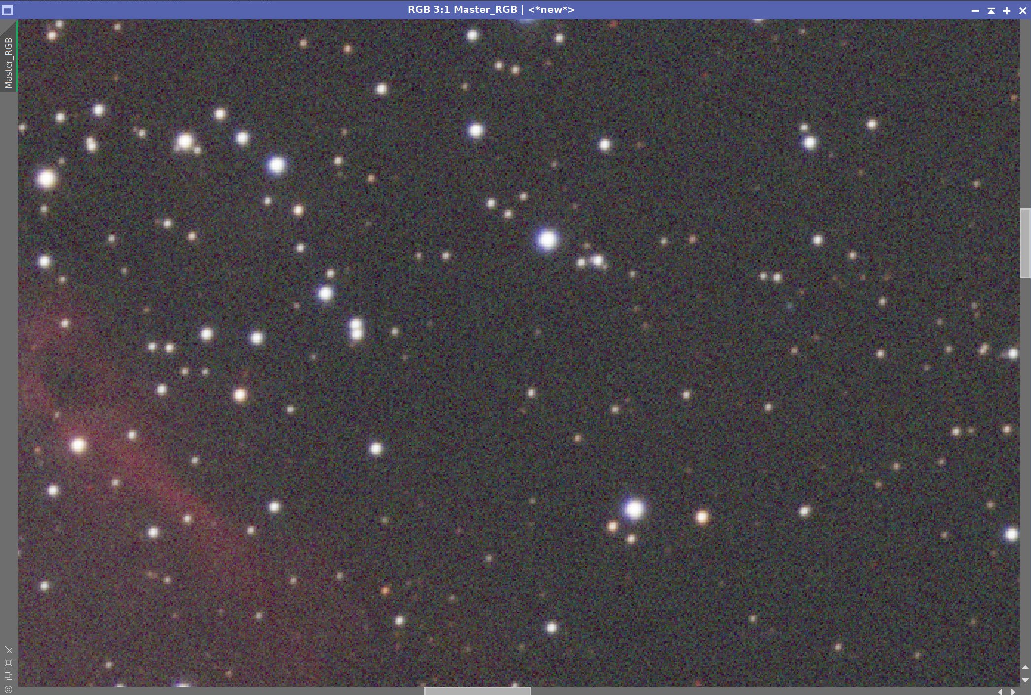
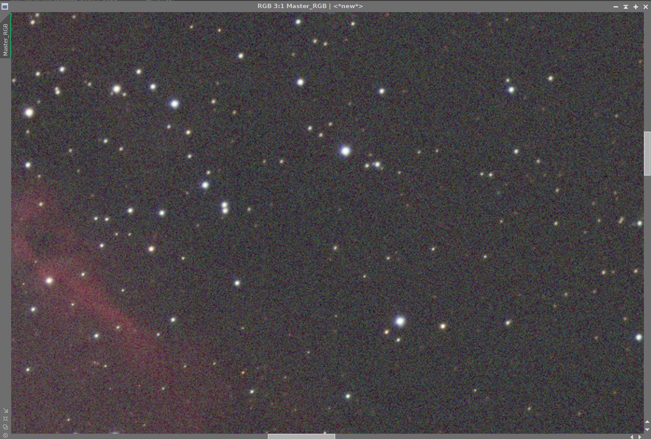
Master RGB (click to enlarge)
4. Run DBE on the Master Images
I will run DBE on the Master SHO and Master RGB images. I probably don’t really need to do this for the RGB image - as I am only going to use it just for the stars - but I thought gradient removal might still help STX to do a better job of star removal, so I chose to do it for both.
DBE was run in subtraction mode.
DBE Sample Pattern for SHO Master (click to enlarge)
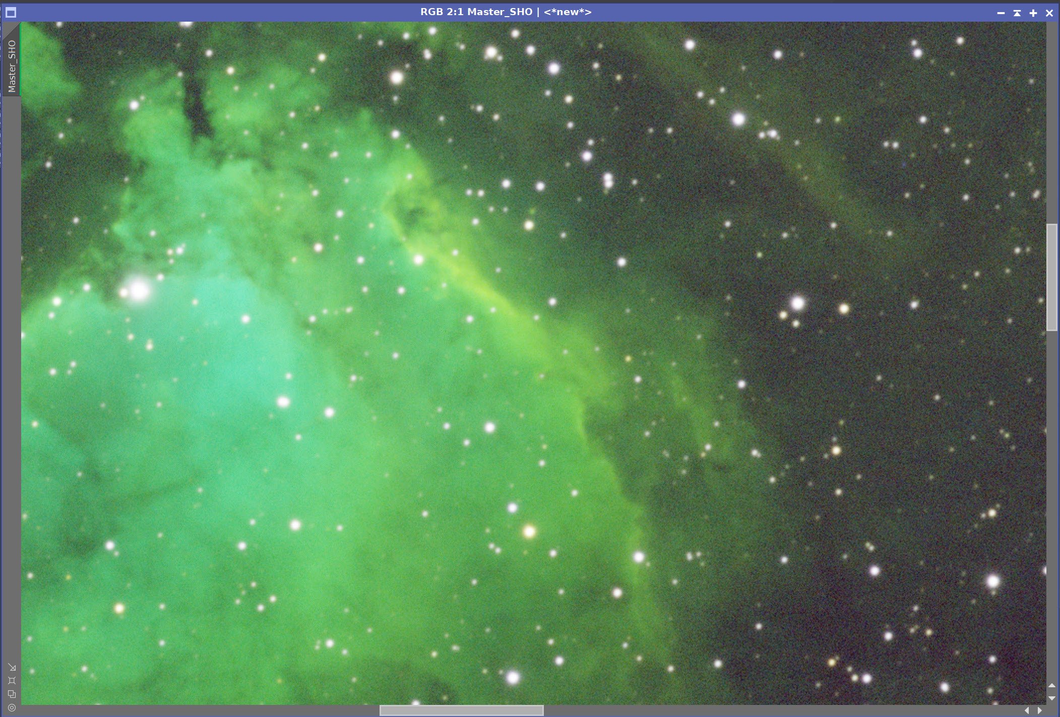
Before DBE for SHO Master (click to enlarge)
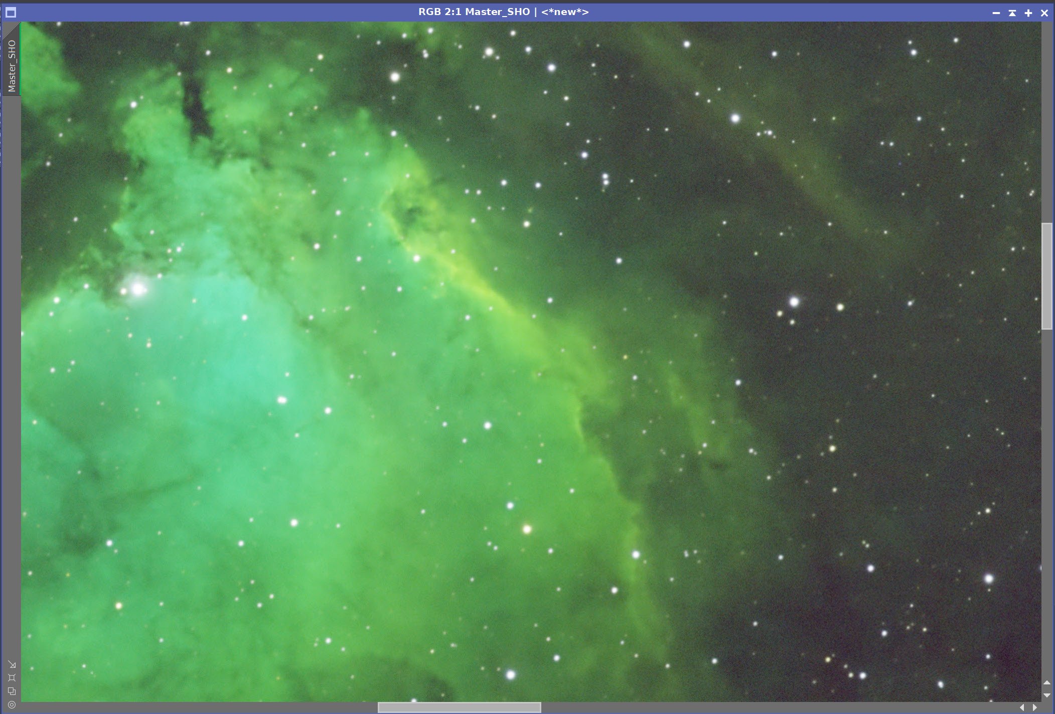
After DBE for SHO Master (click to enlarge)
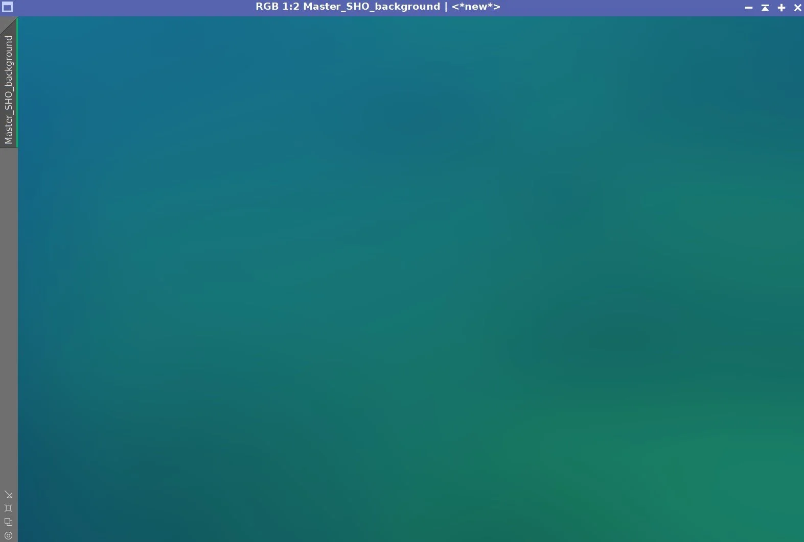
Background Pattern - SHO Master (click to enlarge)
DBE Sample Pattern for RGB Master (click to enlarge)
Before DBE for RGB Master (click to enlarge)
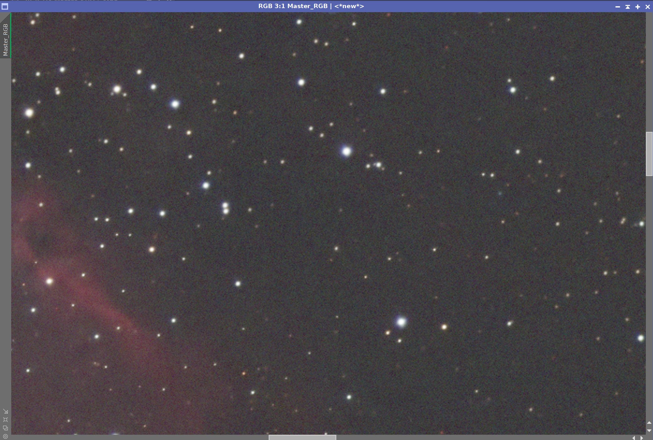
After DBE for RGB Master (click to enlarge)
Background Pattern - RGB Master (click to enlarge)
5. Complete the Linear Processing of the RGB Image
Do a Color Calibration
Select a preview sample of the background sky
Setup SPCC panel
Run SPCC
Run Deconvolution
RUN PFSImage. Whfm X = 2.94 Y = 2.56 - I realized that I did not need to do this, as I had no intention of using the starless nebula data - so instead, I just experimented with the star value and did “Auto” for the nonstellar.
Experiment with values - see panel snap for details.
Run BXT - see panel snap for details
Run Noise Reduction
Run NXT with a value of 0.55

Starting RGB image - note the preview sample area - along with the setup of the SPCC panel.

SPCC Output with the regression line. Note the strange cluster in the top curve - not sure what is going on there!
Master RGB after SPPC (Click to enlarge)


The BXT Panel Setup for the final run
Master RGB Image Before BXT, After BXT, and after NXT = 0.55
6. Do the Linear Processing for the SHO Image
Run PSFImage to determine star sizes: X=3.08, Y= 2.7
I will be using the smaller value - because I assume that we will have any aberrations causing eccentricity removed in the correct first aspect of the BXT run
Run Deconvolution
Experiment with different values
Run BXT - see panel snap for details
Run Noise Reduction
Run NXT with a value of 0.55

The Output from PSFImage for the Master Ha image.

How the BXT tool was configured for the Master Ha image

The Master SHO Image before BXT, After BXT, and After NXT=0.55
7. Go Nonlinear and Create Starless/Stars-Only Images
For the SHO and RGB images, go starless
Preserve the stars for the RGB
Preserve the starless version for SHO
Then go Nonlinear using the STF->HT method
Final Master SHO Image (click to enlarge)
Final Master RGB Image (click to enlarge)
Master SHO Starless Image (click to enlarge)
RGB Star Image (click to enlarge)
8. Extract Mono Images from the Nonlinear SHO image
We want to extract the nonlinear versions of the Ha, O3, and S2 images to process them separately and enhance them.
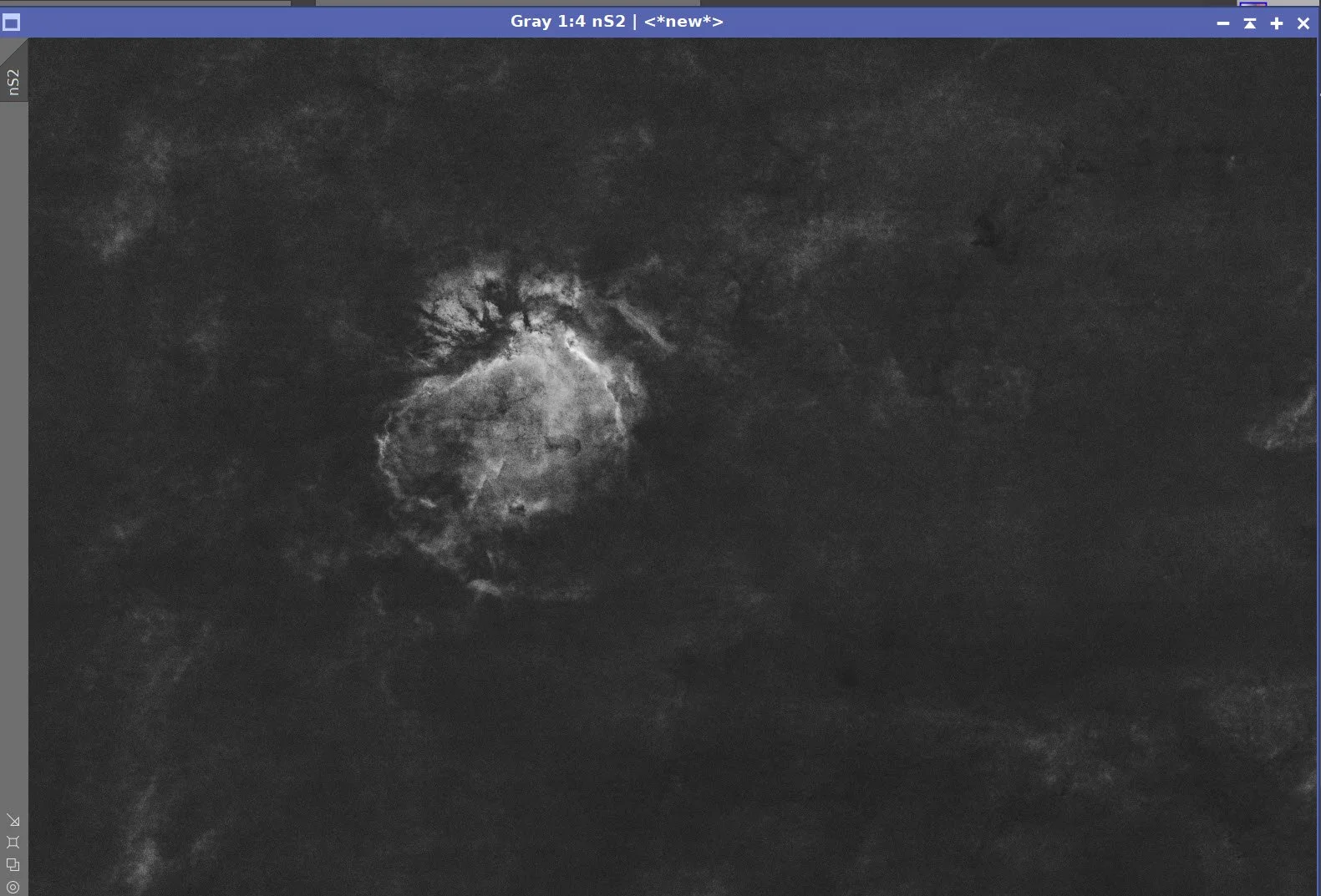
Nonlinear Ha (click to enlarge)
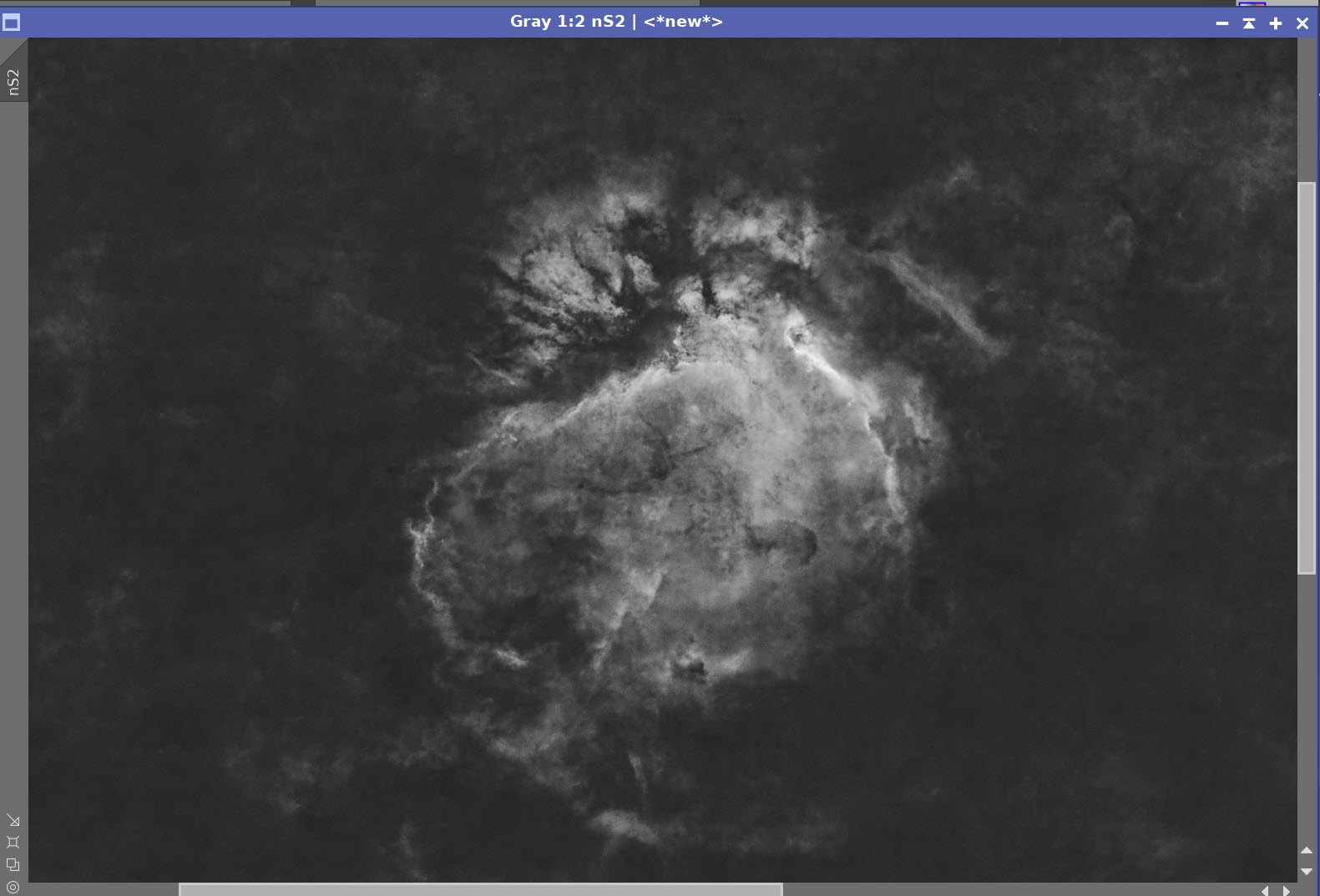
Nonlinear O3 (click to enlarge)
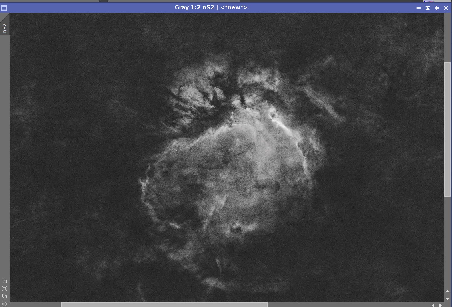
Nonlinear S2 (click to enlarge)
9. Create the Masks That Will Be Used for Processing the Nonlinear Mono Images and the SHO Color Image
Create the Ha_Range_Mask using the Range Selection Tool on the Ha Image
The goal here is to focus on the key signal areas, so this is a kind of subject mask

Ha_Range_Mask
Create the Range_Mask_O3:
Use SelectRange on the O3 image to create a mask that isolates the main area of nebulosity
Clean up the bright corner in the upper left with DynamicPaintBrush
Do further cleanup with CT to bury the noise
Finalize the mask by softening it up a bit with convolution
Inital O3 range mask (click to enlarge)
O3 Range Mask after CT to clean things up a bit more (click to enlarge)
Clean up with the DynamicPaintBrush (click to enlarge)
Soften with Convolution (click to enlarge)
Create Range_Mask_S2
This is a similar range mask but is based on S2 Image data.
This was done completely with SelectRange tool
Range_Mask_S2
Create the WarmTones_Mask
Using ColorMask_Mod, create a mask from color vectors 328 to 48 on the SHO image after the initial color correction
Adjust with CT
Soften with Convolution
Do a final adjustment with CT
Initial WarmTones Mask (Click to Enlarge)
Soften with Convolution (click to enlarge)

Increase the contrast with CT (click to enlarge)
Finish with a final CT Adjustment (click to enlarge)
Create the BlueMask
Run the Color_Mask_Mod tool on the SHO Image and create the BlueMask

BlueMask
Create the OrangeMask
Use Color_Mask_Mod to create a color mask with a hue vector of 12 to 73 and use the initial color-adjusted SHO image.
This captures the brighter orange colors in the image.

OrangeMask
Create the BlueCornerMask
Use Color_Mask_Mod to create a blue mask with the hue from 159 to 277 as run on the color-corrected SHO Image
Use the DynamicPaintBrush to get rid of the central nebula
Apply CT to boost it a bit
BlueCornerMask Initial version (Click to enlarge)
After CT Boost (click to enlarge)
After DynamicPaintBrush reomval of main nebula. (click to enlarge)
10. Process the Ha Image
Apply a global CT to adjust the Tone Scale
Apply HDRMT with levels=7 and “To Lightness”
Apply CT to bring back some of the contrast loss from the previous step
Apply the HARange_Mask
Run LHE with a Radius of 30, contrast limit of 2.0, amount of 0.25, and 8-Bit Histogram
The initial Ha Nonlinear Image (click to enlarge)
After HDR_MT at level 7 to reduce the high-end contrast. (click to enlarge)
After a global CT (click to enlarge)
After a Global CT to restore some contrast lost in the last step (click to enlarge)
The final Ha image after LHE with the HA_ Range_Mask in Place (click to enlarge)
11. Process the O3 Nonlinear Image
Apply. a Global CT to adjust the tone scale
Apply HDR_MT at level 7 and “To Lightness” to compress high-end tone scale
Apply the Range_Mask_O3
Run LHE with radius 64, contrast limit =2, amount = 0.39, 8-bit histogram
Run NXT 0.9
Invert the Range_Mask_O3
Run NXT = 0.63
Final CT to adjust the Tone scale
The Initial O3 Nonlinear Image (click to enlarge)
After a HDR_MT (click to enlarge)
After running LHE with the Range_Mask_O3 (click to enlarge)

After a global CT adjust (click to enlarge)
After another global CT adjust (click to enlarge)
NXT = 0.9 with RangeMaskO3 (click to enlarge)
After NXT = 0.63 with RangeMaskO3 inverted (click to enlarge)
After Final global CT. (click to enlarge)
12. Process the S2 Image
Adjust the image tone scale with CT
Apply RangeMask_S2
Apply LHE with a radius of 64,contract limit = 2.0 ,Amount = 0.3, and use an 8-bit histogram
Run NXT with no mask and a value of 0.68
Finalise with a last CT
Inital Nonlinear S2 image (click to enlarge)
Apple LHE with RangeMask2 (click to enlarge)
After global CT adjust (click to enlarge)
Before and After NXT = 0.68
After Final CT (click ot enlarge)
13. Create the Nonlinear SHO Color Image And Process It.
Use Channel Combination to create the new SHO Image.
Run SCNR Green at 0.9 - this removes the main green color balance
Invert the image - this allows any weird magenta issues to be seen as green.
Run SCNR Green at 0.9 - this easily corrects for magenta issues as SCNR does not support Magenta correction.
Invert Again
Run CT to adjust tone scale, color, and saturation
Apply WarmTones_Mask
Apply CT - adjust tone scale, and color sat
Apply BlueMask
Apply CT - adjust tone scale, and color sat
Apply CT globally
Apply OrangeMask
Apply LHE with a radius of 298, contract limit =2.0, amount = 0.18, and a 12-bit Histogram
MLT sharpening - see screen panel snapshot for parameters
Run NXT 0.68 globally
Apply BlueMask
Appy CT to enhance colors
Do a global contrast adjust with CT
Apply the BlueMask
Apply CT - adjust tone scale, and color sat
Apply BlueCornerMask
I did not like the look of the weird blue in the corner. So I took an artistic license and decided to mitigate it.
Apply CT to smooth out the weird blue corner.
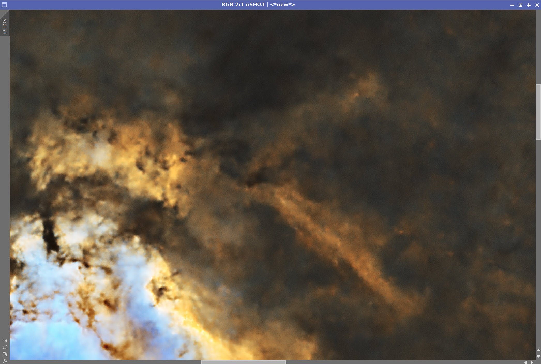
Intiail SHO image (click to enlarge)
Invert the Image(click to enlarge)
Invert the image (click to enlarge)
After CT with Orange Mask (Click to enlarge)
after CT Global (click to enlarge)
After MLT Sharpening with the Orange Mask - See panel snap (click to enlarge)
After SCNR G at 0.9 (click to enlarge)
After SCNR G at 0.9 (click to enlarge)
After global CT (click to enlarge)
After CT with BlueMask (click to enlarge)
After LHE with the Orange Mask (click to enlarge)


Before and After NXT = 0.68
After Global CT (click to enlarge)

After CT with BlueCornerMask (click to enlarge)

CT with BlueMask (click to enlarge)
14. Process the Nonlinear RGB Stars
Tweak with CT to reduce neutral contrast to shrink stars and increase color saturation

Initial Nonlinear RGB Stars

After CT Adjust

The CT curves used for this.
15. Add the SHO Starless and The RGB Stars Images Togther
Using the ScreenStars script, add the stars back in

Combined Image
16. Export the Image to Photoshop for Polishing
Save the image as Tiff 16-bit unsigned and move to Photoshop
Adjust with Clarify and Color Mixer
Do a final curves
Add watermarks
Export Clear, Watermarked, and Web-sized jpegs.

Adding the next generation ZWO ASI2600MM-Pro camera and ZWO EFW 7x36 II EFW to the platform…