
SH2-82 - The Little Cocoon Nebula - 7.3 Hours in LRGB
Date: July 31, 2024
Cosgrove’s Cosmos Catalog ➤#0132

SH2-82 - My first image of the year… sadly! (Click for Full Res Version via Astrobin)
Awarded Flickr “Explore” Status!

Table of Contents Show (Click on lines to navigate)
Back in the Saddle!
Given all of the distractions from the move and the work on the observatory—added to the weather—this is my first image with new data done this year! It is also the image shot at my new location!
Before the move, I set my scopes up in the driveway using my scope Lifter/Mover.
After the move, I had to deal with two things:
The opportunity to build my long sought-after observatory! (Yay!)
A driveway that was no longer suitable for telescope work! (Boo!)
While the prospect of having my observatory is exciting, I have to deal with my new situation. In the interim, I cannot shoot from my driveway (trees and neighbors' lights). The best location now is up the hill in my backyard, where the observatory will go!
However, the scope Lifter/Mover will not make it up the hill, so for right now, I can only haul my smaller Askar FRA400 Rig up for imaging. More on that later!
About the Target
SH2-82 is also known as Bernes 17, LBN 129, LBN 053.54+00.04, DG 159, and Magakian 797. It is also known as The Little Cocoon Nebula (due to its resemblance to IC 5146 - The Cocoon Nebula) and The Little Tridid Nebula (as it also looks a bit like Messier 20 - The Trifid Nebula)
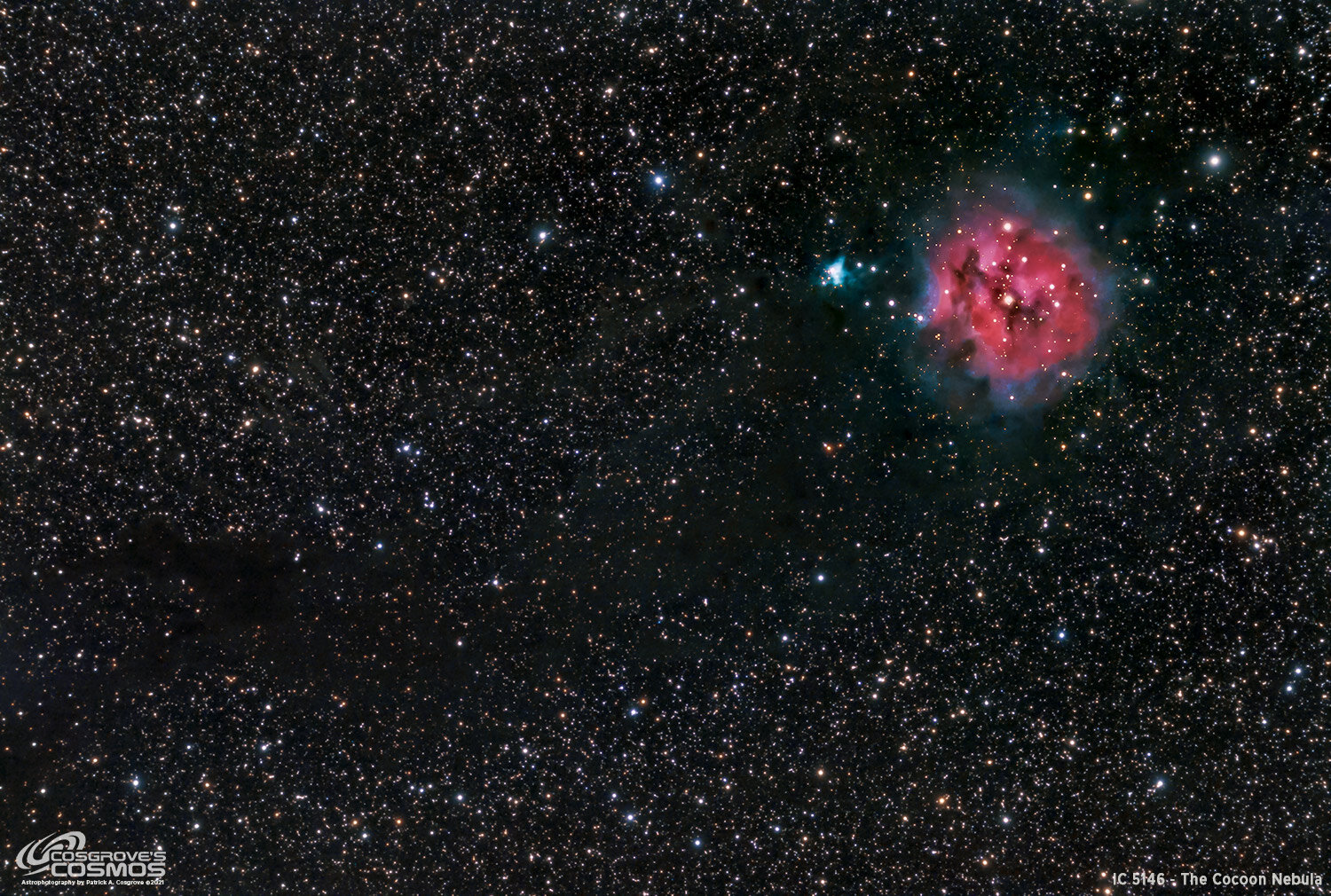
One of my shots of the IC 5146 - Cocoon Nebula

My shot of M20 - The Trifid Nebula
It is both an emission and reflection nebula located about 3950 light-years away in the constellation of Sagitta - The Arrow.
The pink-red portion of the nebula gets its color from the emission of photons from hydrogen gas ionized by the B0.5V star HD 231616. Based on its distance estimate, it appears to be near the Vulpecula OB4 association.
This region is known as an area of rapid star formation. It is surrounded by a slightly blueish area made of dust that glows from reflected light.
The entire region is in a very rich portion of the Milky Way, loaded with stars and glowing gas. Areas of dark dust—nodules and streaks—can also be seen near SH2-82 and in the general neighborhood.
This target is not that well known and is infrequently imaged. In fact, I could not find much information about this target - which made it all the more attractive to me!
The Annotated Image

This annotated image was created using the Imagesolver and AnnotateImage capabiliites found in Pixinsight.
The Location in the Sky

This annotated image created with Imagesolver and Annotate Image Scripts in Pixinsight.
About the Project
A while back, I had my first clear night in the new location after the move, I tried hauling the Ask FRA400 platform up the hill for a first night of imaging.
This effort turned out to be a bit of a disaster!
It was my first time trying to figure out how to make things work in the new property, and all I had were problems. The gear had been through a move and had not been used for a while. Things did not go well:
Endless software updates on my control computer
Loose focus motor coupler issues causing auto-focus failures
USB connection issues
The camera Rotator moving in the WRONG direction
Tracking issues
The end result - no data and much frustration. I had to wait for this imaging project to get things sorted out!
Picking the Target
The second time I had a chance to collect data was on July 6 of this year.
So I looked at what constellations would be well poised on the eastern tree line and went to Astrobin so I could review images taken from those constellations.
I came across SH2-82 and I thought it looked kinda cool. I had never heard of this object before, but I liked the combination of red glowing gas and all of the dark nebulae around the area. Most of the images I saw of it were a bit crude, and I wondered if I could do better.
As I said before, it is infrequently imaged, and there is not much information about it. I love targeting lesser-known objects!
I determined how to frame the image and set things up in Sequence Generator Pro so I was ready to grab data.
Data Collection
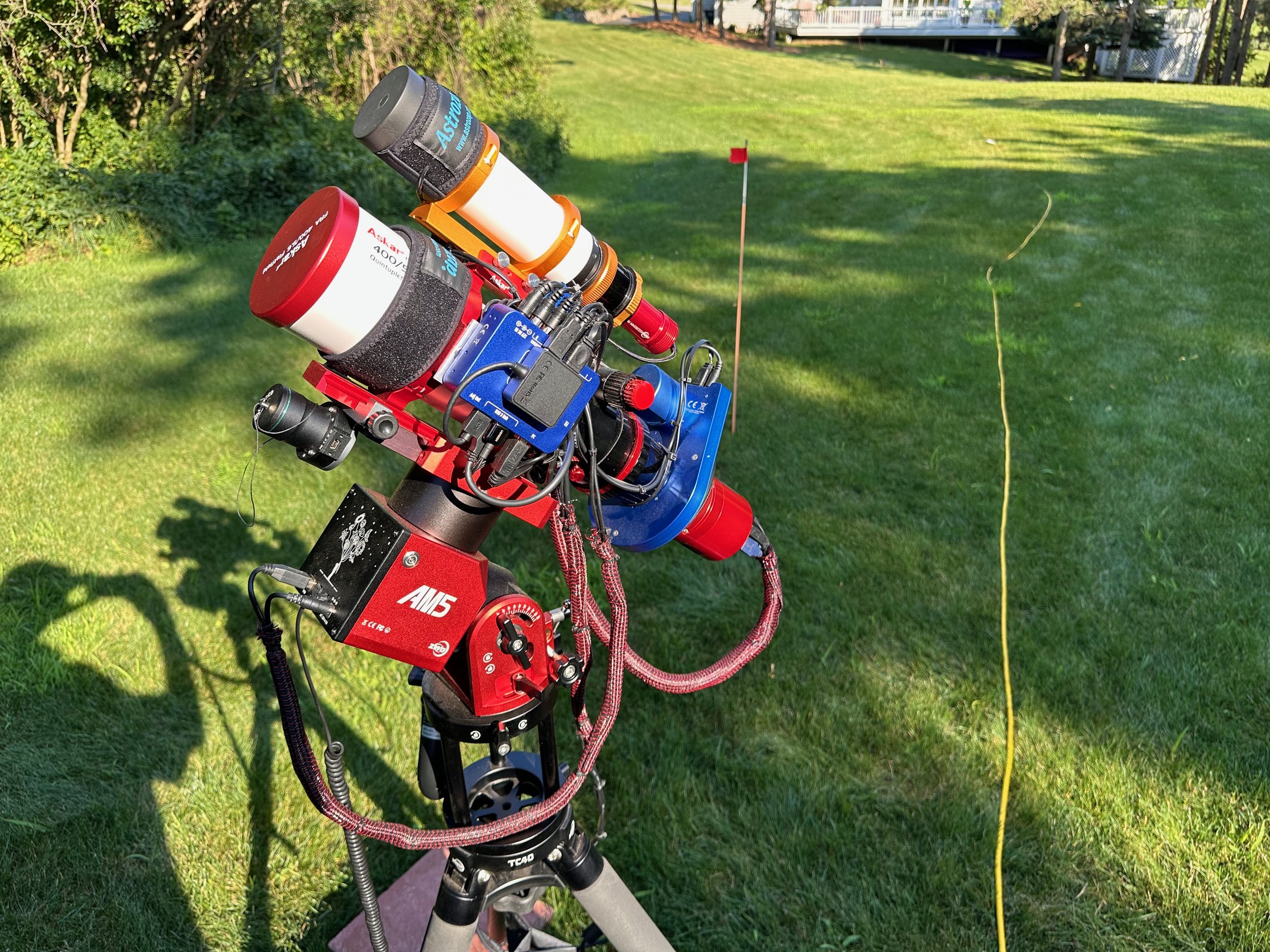
I set three patio blocks up on the hill in my backyard. Then, I hauled up a folding table and a folding chair. I slung two 50’ extension cord reels and a section of 100’ extension cord to get power up there.
Then I hauled the Askar FRA400 platform up the hill (Damn, I am getting old - this thing seemed heavier than it did last year!)

As I set things up, this time, I ran into no trouble.
We had a pretty clear night with a hint of thin clouds late in the evening.
I ended up collecting 4 hours of LRGB 90-second subs for this target!
The next morning, I set the rig up in the garage and captured fresh Darks, Flats, and DarkFlats! Its been a while since I did any images, and I wanted fresh cal data.
It turns out I had a problem with what I did here, and I did not find out until much later.
I then tried integrating the data with WBPP - and discovered a few things:
This was faint data. I really needed more integration time.
The noise seemed worse than expected. I am using the older 1600 mono camera on this rig and not the 2600 I have on the other rigs. Boy, how I wished I had the newer 2600 here!
I had horrible walking noise on my Blue Master Image.
I was not sure what happened with the Blue Master - perhaps my dithering got disabled? I realized I would have to recollect the blue data for this project to proceed.
On July 26 I had another clear night - at least until the quarter Moon came up, so I set things up again and collected another set of blue data with maximum dithering - and I verified that my dithering was working!
Unfortunately - the wildfires in Canada and out west were active again, and we were beginning to get some smoke in the upper atmosphere.
These days, I seem to spend as much time watching smoke patterns as clouds! On this evening the smoke was predicted to be minimal but in the following days it would become much worse - so I needed to capture my photons while the “gettin’ was good.”
I also ended up collecting about another 3 hours of LRG along with the B data until the Moon came up.
So now I could reprocess all of my data.
Once Again - walking Noise on the Blue channel! What?!
Data Analysis - Not Following My Own Rules!
I knew I had the dither right.
Why only the blue channel?
I started to suspect that what I was seeing was not a dither problem at all. if I had walking noise with my blue filter, why not on the other subs with the other filters? They would have all had the same level of dithering.
So I looked at how I had WBPP setup and realized that there were NO blue dark flats in my data set! WBPP gave no warning about this - which is odd.
What happened to my Blue Dark Flats?
Then I looked at my flats. I saw that I had twice as many Blue Flats as the others. Hmmmm.
I blinked my Flats, and I found that I had one set of Flats and one set of DarkFlats labeled as Flats!
I looked at the sequence file for SGP that I used to create the cal files and noticed that I had the DarkFlats for blue mislabeled as Flats, not Darks!
OOPS!
So, my blue problems were caused by having DarkFlats mixed into my flat computations and no DarkFlats at all for calibration.
I fixed this problem, reran WBPP, and low and behold - nice, clean master images.
I have always had a hard and fast rule:
Always, Always blink every subframe of light, dark, flats and darkflats data collected!!
In my hurry to see my first image data in a long time, I skipped this step for the cal data. Mistake!
Had I done this step, the problem would have been obvious, and I could have fixed it much sooner. So, live and learn. I adopted my rules for good reason - I need to follow them!
However, I had done a blink analysis on all the Light images, and the data generally looked quite good. I did see a surprising number of satellite and meteor trails, but I knew that the integration rejection logic would handle them well.
The signal was very low, and I was hoping my 7.3 hours of integration would be enough to do the target justice, but I had my doubts. I really need a lot more integration. However, with the smoke patterns and weather, this was unlikely. In fact, I was not able to collect more data for this target.
Image Processing
I tend to do a lot of narrowband work, and in this case, I decided to go LRGB in order to get the reds of hydrogen clouds as a backing. So I needed to do a LRGB workflow.
I was also planning on doing a Starless Workflow, so I could really work on the nebulae. Given the density of stars in this region, I was not sure how this would work out, but I was committed to trying this path.

My Workflow for this image
For this image, I was also looking forward to trying out a few new scripts that have become available recently. The AutoDBE script by Seti Astro, and the ImageBlend script by Mike Cranfield. The latter I would use as a replacement for LRGBCombination. So I was excited to see how this would work out for me.
Final Results
It’s been a LONG time since I had some fresh data to work with, and I have to say, doing this project was a lot like coming home after you have been away for a long time! It felt great!
This is such a faint target that, given the limited integration, bringing out its features was a real challenge.
I also noted that StarXTerminator was really challenged by this image. It still did a wonderful job, but it did leave behind some blemishes around brighter stars that I did not like. I suspect that I had some light clouds the first night and some smoke the second night, and this may have added to the challenge.
Having said that, I was still reasonably pleased with the final product. It is not my best image, but it certainly is much better than my worst image!
Look below for the complete step-by-step processing walkthrough! Note: This walkthrough is based upon the use of Pixinsight.
Capture Details
Lights Frames
Taken the nights of July 6th and 26 , 2023.
88 x 90 seconds, bin 1x1 @ -15C, Gain 100.0, Astronomiks ZWO L Filter - 1.25 inch
56 x 90 seconds, bin 1x1 @ -15C, Gain 100.0, Astronomiks ZWO R Filter - 1.25 inch
56 x 90 seconds, bin 1x1 @ -15C, Gain 100.0, Astronomiks ZWO G Filter - 1.25 inch
91 x 90 seconds, bin 1x1 @ -15C, Gain 100.0, Astronomiks ZWO B Filter - 1.25 inch
Total of 7 hours and 16 minutes and 30 seconds.
Cal Frames
25 Darks at 300 seconds, bin 1x1, -15C, gain 100
25 Dark Flats at Flat exposure times, bin 1x1, -15C, gain 100
One set of Flats done:
12 L Flats
12 R Flats
12 G Flats
12 B Flats
Capture Hardware
Scope: Askar FRA400 72mm f/5. 6 Quintuplet Air-Spaced
Astrograph
Focus Motor: ZWO EAF 5V
Guide Scope: William Optics 50mm guide scope
Guide Scope Rings: William Optics 50mm slide-base Clamping Ring Set
Mount: ZWO AM5
Tripod: ZWO TC40 Carbon Fiber tripod w/160mm Extention
Camera: ZWO ASI1600MM-Pro
Camera Rotator: Pegasus Astro Falcon Camera Rotator
Filter Wheel: ZWO EFW 1.2 5x8
Filters: ZWO 1.25” LRGB Gen II, Astronomiks 6nm Ha, OIII,SII
Guide Camera: ZWO ASI290MM-Mini
Dew Strips: Dew-Not Heater strips for Main and Guide Scopes
Power Dist: Pegasus Astro Powerbox Advanced
USB Dist: Pegasus Astro Powerbox Advanced
Polar Alignment
Cam: PoleMaster
Software
Capture Software: PHD2 Guider, Sequence Generator Pro controller
Image Processing: Pixinsight, Photoshop - assisted by Coffee, extensive processing indecision and second-guessing, editor regret and much swearing…..
Click below to visit the Telescope Platform Version used for this image.
Image Processing Walkthrough
(All Processing is done in Pixinsight - with some final touches done in Photoshop)
1. Blink Screening Process
Lum
many satellite trails, no rejects
Red
many satellite trails, no rejects
Green
many satellite trails, no rejects
Blue
many satellite trails, no rejects
Flats (when I finally viewed them…)
All fine, but Blue had a mix of flats and darks by accident. This was corrected.
Dark Flats
Missing - but then restored - they looked fine.
2. WBPP 2.7.3
Reset everything
Load all lights
Load all flats
Load all darks
Select - maximum quality
Reg reference - auto - the default
Select the output directory to wbpp folder
Enable CC for all light frames
Pedestal value - auto for all NB filters
Darks -set exposure tolerance to 0
Lights - set exposure tolerance to 0
Lights - all set except for linear defect
Integration - large-scale rejection layer 2x2
set for Autocrop
Set cosmetic corrections for all
No Drizzle
Executed in 59:26

WBPP Calibration View

WBPP Post Calibration View

WBPP Pipeline View
3. Load Master Images
Load all master images and rename them.
Create an initial RGB Image using ChannelCombination

Master L Image

Master R, G, and B images - and the combined Master_RGB image.
4. DBE
Used AutoDBE script for the first time
Run for the Master L image after selecting avoidance zones for the main nebula and its dark components.
Run for the Master RGB image after selecting avoidance zones for the main nebula and its dark components.
This is pretty easy to use - but I need more experience with it before I can say it is my new goto DBE tool.

The Panel settings used for the Master L image
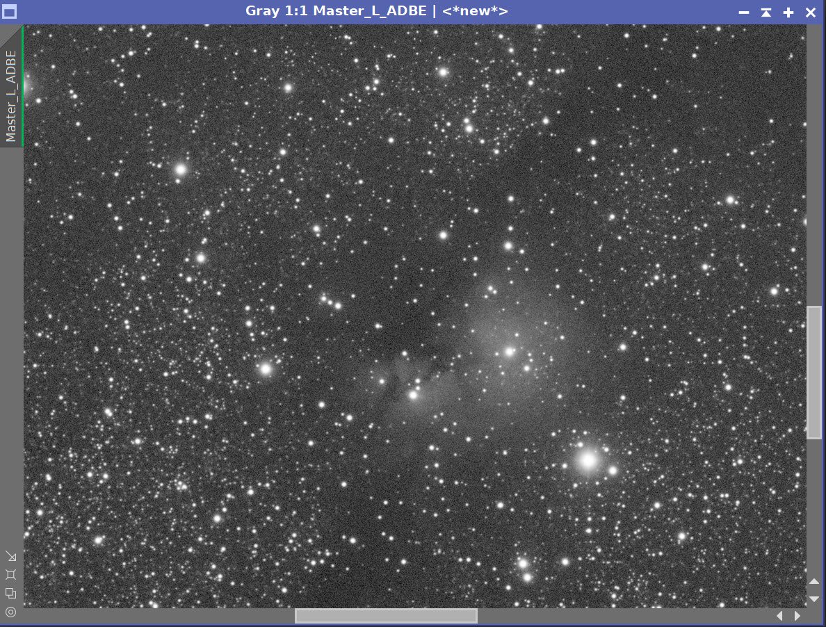
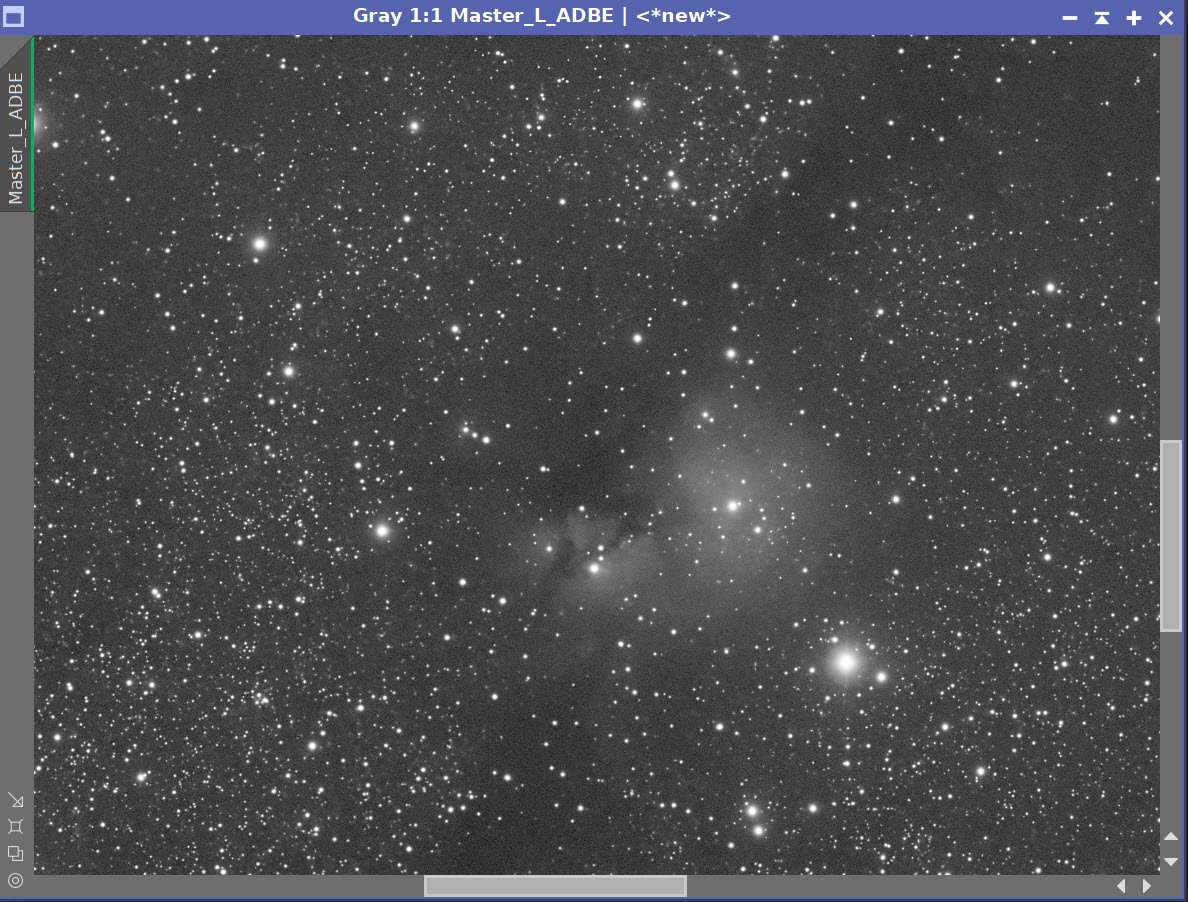
Master_L Before AutoDBE (click to enlarge)

Master_ L after AutoDBE (click to enlarge)

Master_L Background

The panel settings used for the Master_RGB image
Before AutoDBE for the Master RGB (click to enlarge)
After AutoDBE for the Master RGB (click to enlarge)
The background image subtracted (click to enlarge)
5. Run SPCC on the Color Image
Setup the SPCC panel using a preview selection rectangle that corresponds to the darkest part of the image.
Run SPCC
Note that the curve fit show some nonlinearites so expect so color issue at the extremes.

SPCC Panel Setup
UPDATE: One of my sharp-eyed readers noticed something strange with my panel shot of the SPCC tool. Filters chosen were for the Sony Color Sensor. I should - of course - used the ZWO R, G, and Blue Settings. Why did I not? simple - I screwed up! This probably explains the curve. Somehow - through sheer dumb luck - it did not cause a bigger issue for me. Maybe if it had, I would have noticed and corrected this before going forward. Apparently, Astrophotography can tolerate the occasional bone-head move…

The regression analysis. Note the nonlinearities.
Master RGB before SPCC (click to enlarge)

Maser RGB After SPCC (click to enlarge)
6. Run BlurXterminator on the L and RGB Images
Process L image:
Run PSFImage to determine star sizes for the Master L image: X = 2.33 Y = 2.24
I will be using the smaller value - because I assume that we will have any aberrations causing eccentricity removed in the correct first aspect of the BXT run
Run Deconvolution
Run BXT for correction only
Experiment with different values
Run BXT - see panel snap for details
Run Noise Reduction
Run NXT with a value of 0.45 - just taking the “fizz off!”
Process the RGB Image:
Run PSFImage to determine star sizes for the Master L image: X = 2.33 Y = 2.24
I will be using the smaller value - because I assume that we will have any aberrations causing eccentricity removed in the correct first aspect of the BXT run.
Run Deconvolution - Fix Only for
Experiment with different values
Run BXT - see panel snap for details
Run Noise Reduction
Run NXT with a value of 0.45 - just taking the “fizz off!”

The Output from PSFImage for the Master Ha image.

How the BXT tool was configured for the Master Ha image


The Master L Image before BXT, After BXT COrrection only, and After NXT=0.55

PFSImage Results for the RGB Master image

BXT panel setting used for the Master RGB image
The Master L Image before BXT, After BXT COrrection only, and After NXT=0.60
7. Create Starless/Stars-Only Images
Go starless and preserve the star image.
Use StarXterminator to remove stars for both the L and RGB images and create a stars-only image for both the RGB images.
I want to use the RGB data for the stars as the L stars are somewhat bloated. But I will use the nebula details from the L image.
Master L Starless Image (click to enlarge)
Master RGB Starless Image (click to enlarge)
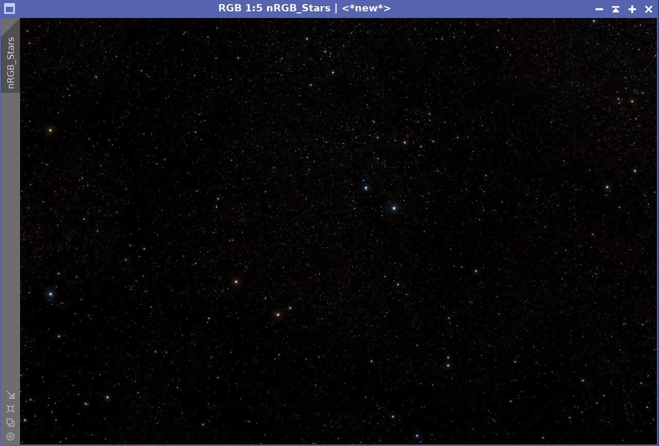
Master RGB Stars Image (click to enlarge)
8. Take RGB Stars Nonlinear and Process
Make a clone of the Master_RGB_Stars image and turn off STF
Use HT to bring the stars just to the point where they look good in the nonlinear domain.
Adjust the stars with CT to reduce stars a bit and to enhance their natural color saturation. Lower the neutral curve and increase the sat curve. See Panel-snap below.

RGB Stars after going nonlinear with HT.
After CT adjust.
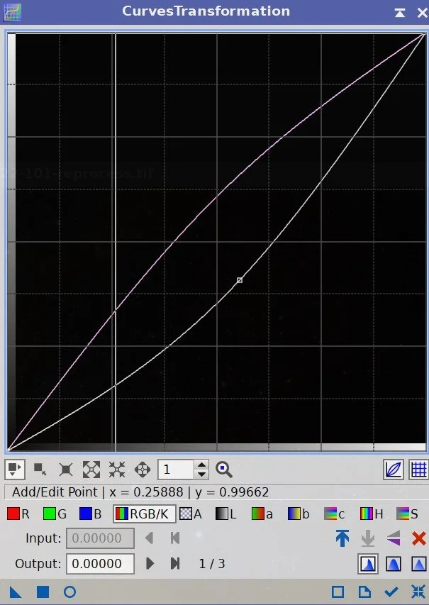
CT panel setting for star adjustment
8. Take the RGB Starless Image Nonlinear and Process It
Use the Seti Astro Statistical Stretch Script to go nonlinear. (See screen snap below)
Apply NoiseXterminator with a value of 0.9. Since this is the starless RGB image we will go aggressive here since the detail will come mostly from the Lum image.
Apply SCNR green to handle some of the background green noise
Apply CT to darken the image to prepare it for combination with the luminance image.

Panel Settings used for the stretch
The Initial RGB Nonlinear Image (click to enlarge)
After NXT = 0.9 (click to enlarge)

After CT applied to enhance color

CT Panel used (click to enlarge)
After SCNR Green applied. (click to enlarge)
Use CT to darken in preparation for Lum image injection. (click to enlarge)
9. Take the Lum Starless Image Nonlinear and DO initial Processing
Create a copy of the linear Lum starless image
Use the STF->HT Method to go nonlinear
Appy NXT with a value of 0.66
Apply CT
Make a copy of the linear Lum image. (click to enlarge)
After NXT = 0.55 (click to enlarge)
Go nonlinear. (Click to enlarge)
Apply CT to set initial contrast (click to enlarge)
10. Create a Lum Range Mask For Selective Processing
Apply RangeSelection to the L_Starless image to create a Lum RangeMask (see screenshot below)
Clean up the mask with CloneStamp and the paint-pot method to create a mask focused on the main object
Initial RangeMask (click to enlarge)

RangeSelection Panel Settings Used.

CloneStamp used to focus the mask on the main target object.
11. Finish Processing the Luminance Image
Make a clone of Lum Starless Image
Apply Rangemask
Apply HDRMT with layers - 6 - this will restore lost detail in the brighter portions of the main nebula.
Appl CT to rebalance the mask area.
Apply LocalHistogramEqualization with scale = 64, contrast limit = 2.0,Amount = 0.5, and 8-bit Histograms
Invert mask
Run NXT with a value = 0.75. This will reduce the noise in most of the image without hitting the main area too hard.
Remove mask
Run Darkstructure script with Default values to enhance the dark lanes.
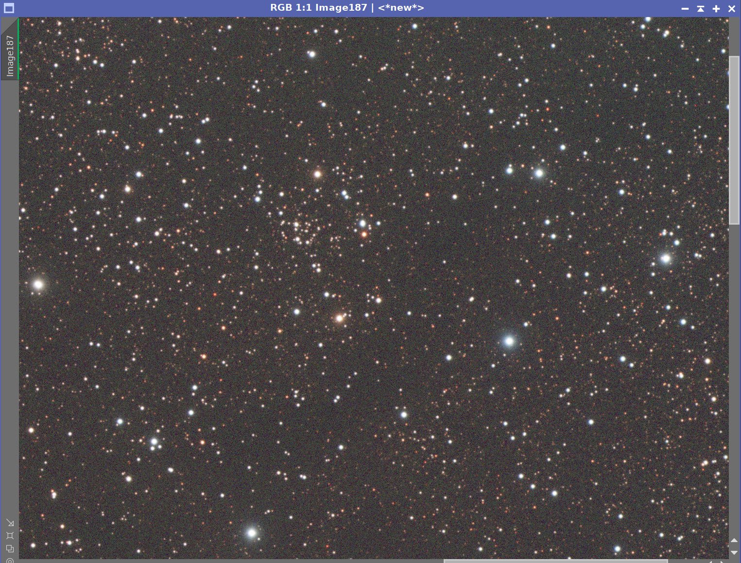
Starting L Starless image (click to enlarge)
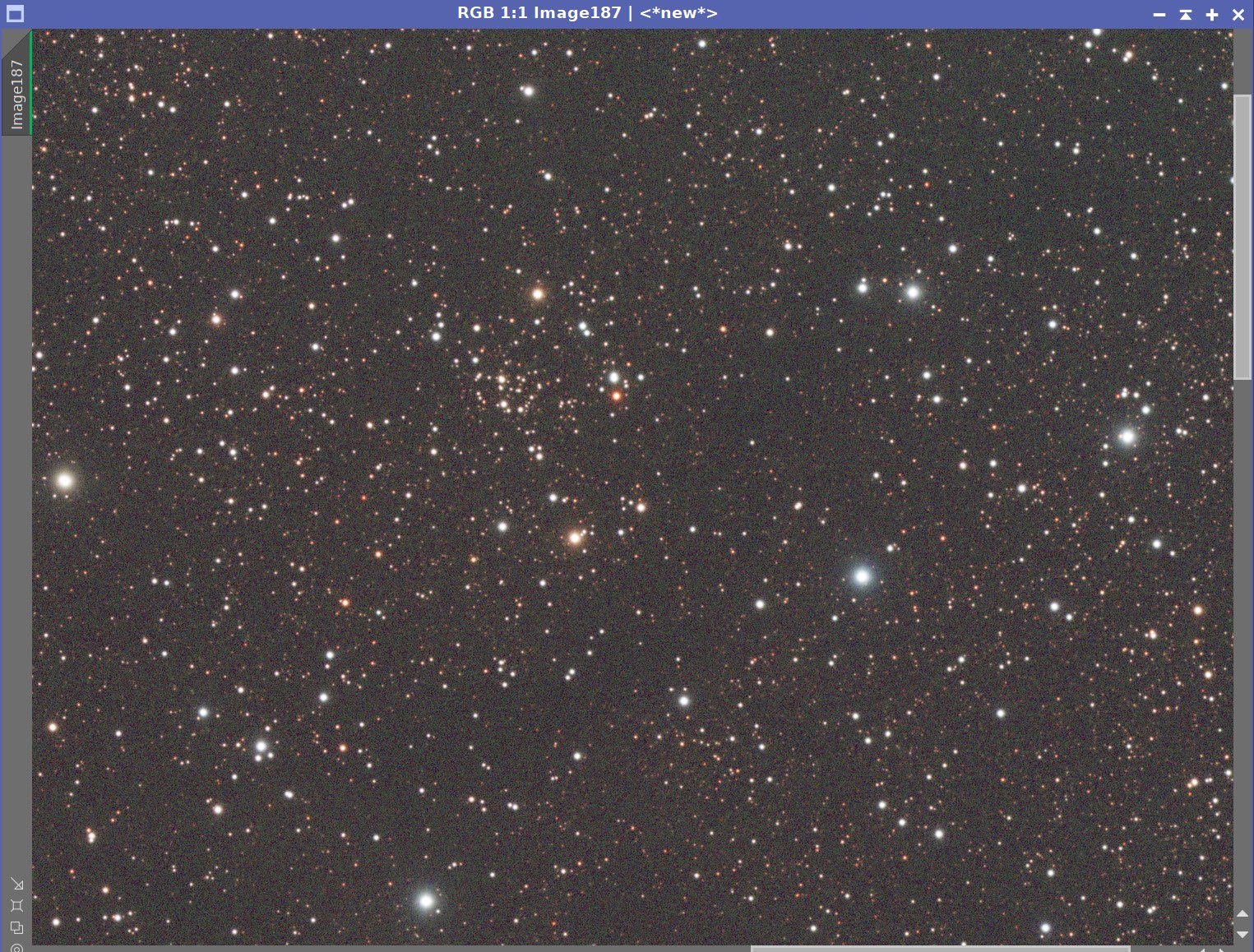
Readjust mask area contrast with CT (click to enlarge)

Run HDRMT with levels = 6 and use the mask (click to enlarge)
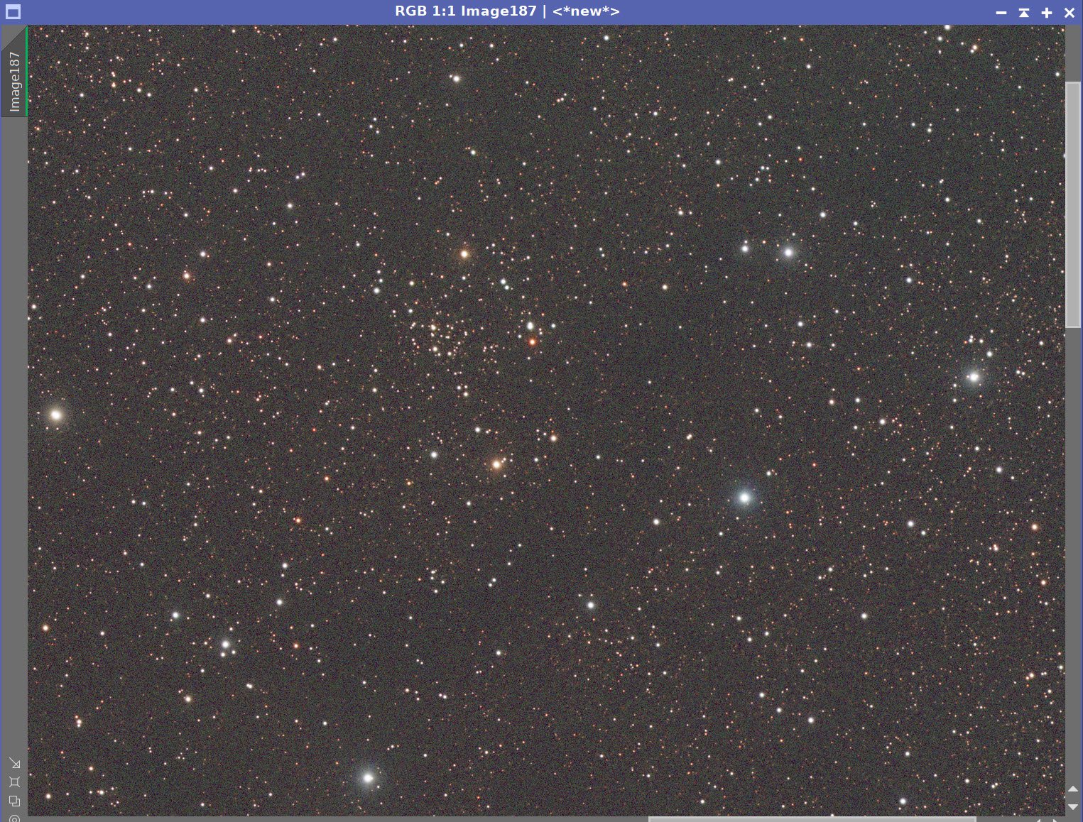
Run LHE to sharpen areas in the mask (click to enlarge)
12. Blend the Lum Starless Image with the RGB Starless Image
Typically I inject the Lum image into the RGB image by using LRGBCombination. I never liked this tool, and I thought I would try the newish script by Mike Cranfield called ImageBlend. This allows you to take two images and blend them together with a variety of methods and controls. It also allows you to do a preview of your method before you commit to a final blend.
In this case, I used the Screen method and played with the opacity control until I liked what I saw. See the screen snap below for what I used.
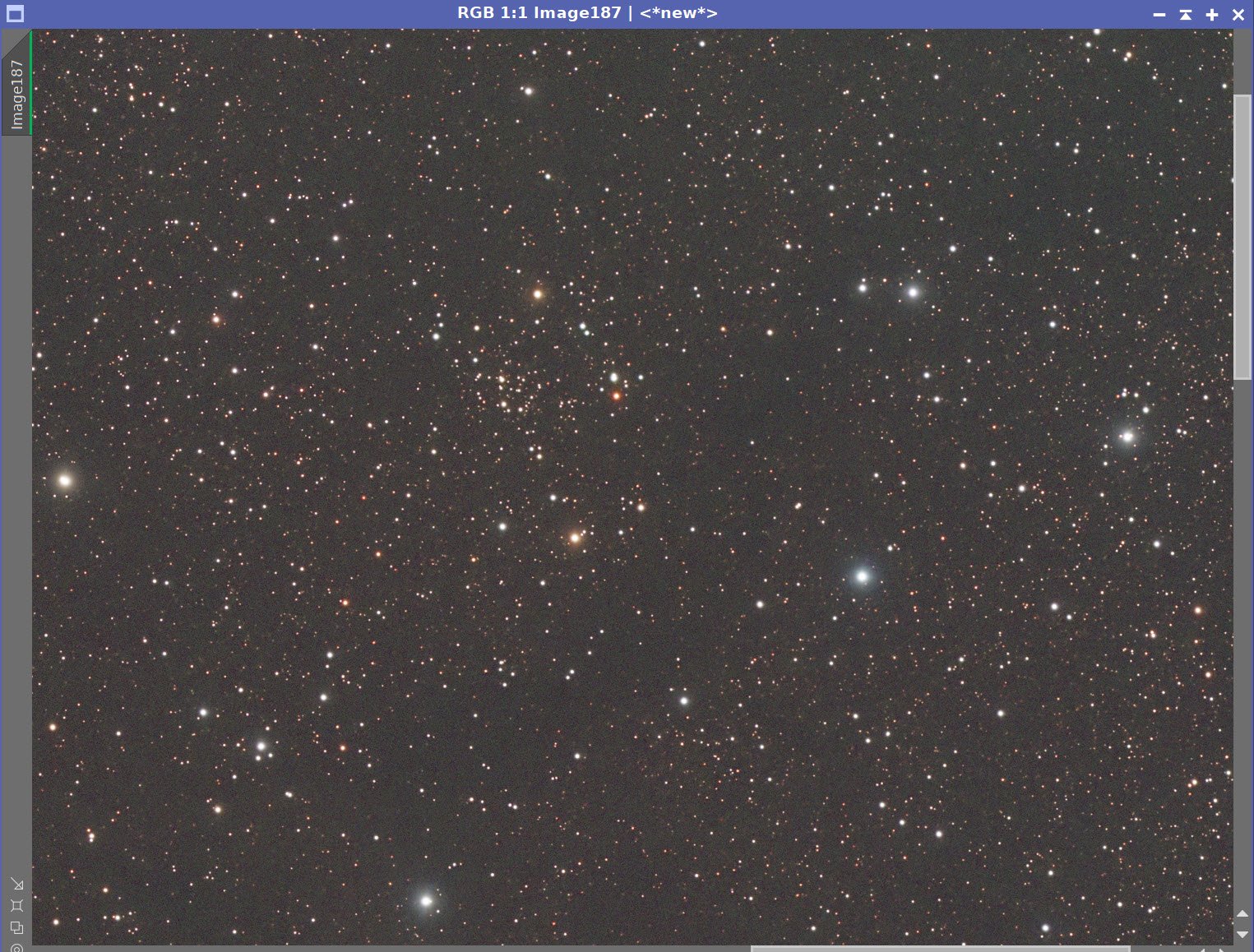
Final Lum Starless Image (click to enlarge)
Final RGB Starless Image (click to enlarge)

ImageBlend Panel settings

The Final LRGB blended starless image
13. Add the Stars Back In and Finish Processing
Use the script ScreenStars to add RGB Stars and LRGB Starless images back together
The Final RGB Stars Image (click to enlarge)
The Final LRGB Starless Image (click to enlarge)

The image with stars!
14. Export the Image to Photoshop for Polishing
At this point, I was pretty happy with the image. Given how noisy the master images were, I thought this was a good result. At this point I usually move to Photoshop and do a little polishing and finishing. However this time, I found that my “polishing” process was a little more involved as you will see.
Save the image as Tiff 16-bit unsigned and move to Photoshop
Do an image crop. This was pretty modest.
Make final global adjustments with Clarify, Curves, and the Color Mixer - these made bigger changes than I normally do.
Using the select tool with a feather of 100 pixels, select some feature areas and use clarity to tweak - I focused efforts here to enhance dark dust detail, the main object detail, and to suppress some subtle halos on some stars.
Add watermarks
Export Clear, Watermarked, and Web-sized jpegs.

The Final Image!
During August and September I was out shooting every clear night. I had learned a lot of things but I was also noticing several issues that were causing me problems as I did more imaging. I decided to do something to address those issues….