November 8, 2026
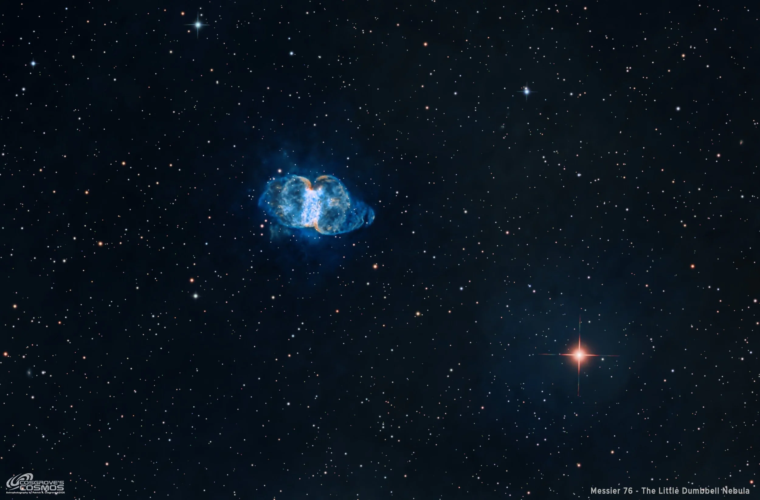
My Image of M76.
This page is the Image Processing Walkthrough page for the Messier 76 (2026) Imaging Project.
🔭 Project Summary
Target: Messier 76 (M76) — The Little Dumbbell Nebula / NGC 650 & NGC 651 / PN G130.9−10.5
Capture Dates: September 6, 11, and 14, 2026
Constellation: Perseus • Distance: ≈ 3,400 light-years
Type: Bipolar planetary nebula — the glowing expelled atmosphere of an evolved star approaching the white dwarf stage
Angular Size: ≈ 2.7 × 1.8 arcminutes, including the extended lobes
Imaging Period: September 6–14, 2026 • Total Integration: 12 h 16 m 30 s (SHO narrowband + RGB stars)
Filters: Ha · OIII · SII (Astronomik 36 mm 6 nm) + R · G · B (ZWO 36 mm LRGB Gen II)
Telescope: Sharpstar SCA260 V2 260 mm f/5.0 Special Cassegrain Astrograph
Camera: ZWO ASI2600MM-Pro (−15 °C; Gain 100 narrowband, Gain 0 RGB)
Mount: iOptron CEM70 on custom steel pier with modified iOptron top pier plate
Guiding: ZWO OAG-L with ZWO ASI174MM-Mini guide camera
Processing: PixInsight (SHO narrowband + RGB stars) & Photoshop
Location: Whispering Skies Observatory · Honeoye Falls, NY (USA)
Acquisition Notes: Ha: 50 × 300 s; OIII: 47 × 300 s; SII: 47 × 300 s; R: 12 × 30 s; G: 11 × 30 s; B: 10 × 30 s, all bin 1×1 at −15 °C. Narrowband exposures used Gain 100; RGB exposures used Gain 0. Total of 177 accepted light frames, providing 12 h 16 m 30 s of integration after culling bad or questionable subs.
Calibration Notes: 25 darks at 300 s, bin 1×1, −15 °C, Gain 100; 25 darks at 30 s, bin 1×1, −15 °C, Gain 0; 30 dark flats at each flat exposure time (Gain 100 for narrowband, Gain 0 for RGB); 15 flats each for Ha, OIII, SII, R, G, and B.
Imaging Challenges: Cloud interference during the three-night imaging campaign required substantial rejection of affected exposures. The surviving RGB data, used primarily for natural-color star rendering, amounted to only approximately one-third to one-half the number of frames normally acquired for this purpose. Despite the reduced RGB integration, the narrowband dataset provided substantial signal for revealing the nebula's complex internal structures and faint outer lobes.
Image Note: This SHO narrowband image with RGB stars captures Messier 76, a compact but remarkably intricate bipolar planetary nebula in Perseus. Its bright central region reveals a complex network of blue-cyan emission, filamentary structures, and warmer-colored knots, while two broad, faint lobes extend outward into the surrounding star field. The apparent rectangular central region is believed to represent a dense equatorial ring viewed nearly edge-on, with the extended lobes tracing material expelled along the nebula's polar axis. The image highlights the striking contrast between the bright inner structure and the delicate outer emissions that reveal the nebula's three-dimensional geometry and evolutionary history.
Table of Contents Show (Click on lines to navigate)
Special Note
Welcome to the new Image Processing Page for this project! If you arrived here from the main Image Project, you can easily return to it using your browser's back button.
Abbreviations Used
Messier 76 — SHO + RGB Stars Processing Flow
Sequential summary of the M76 workflow, following the M76 image processing walkthrough: cloud-related frame culling, WBPP 3.2 integration, SHO and RGB master construction, triangular star correction, linear noise and background processing, nonlinear tone recovery, color correction, selective sharpening, faint nebulosity enhancement, Astro Star Lab recombination, and Photoshop finishing.
Processing this Image
(Most processing was done in PixInsight, with final touches in Photoshop)
1. Blink
Ha
5 frames removed for clouds.
OIII
5 frames removed for clouds.
SII
5 frames removed for clouds.
Red
5 frames removed.
Green
5 frames removed.
Blue
6 frames removed.
Darks
All looked OK
Dark Flats
All looked OK
Flats
All looked OK
2. WBPP 3.2
Reset everything
Load all lights
Load all flats
Load all darks
Select Maximum Quality
Reference Image: Auto (default).
Select the output directory for the WBPP folder
Enable CC for all light frames
Pedestal value - auto
Darks - set exposure tolerance to 0
Lights - set exposure tolerance to 0
Set for Autocrop
WBPP completed in 22 minutes, 14 seconds, with no errors.
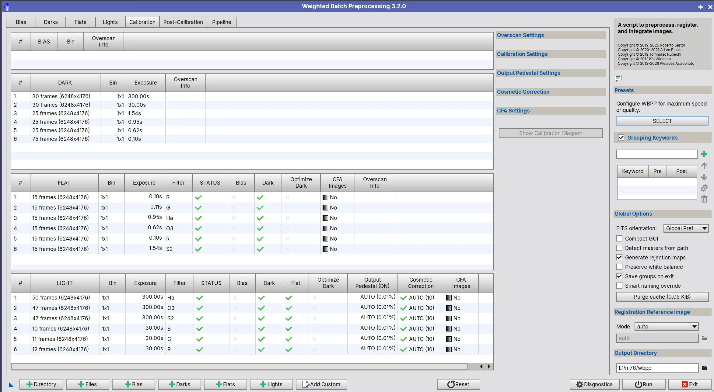
WBPP Calibration View
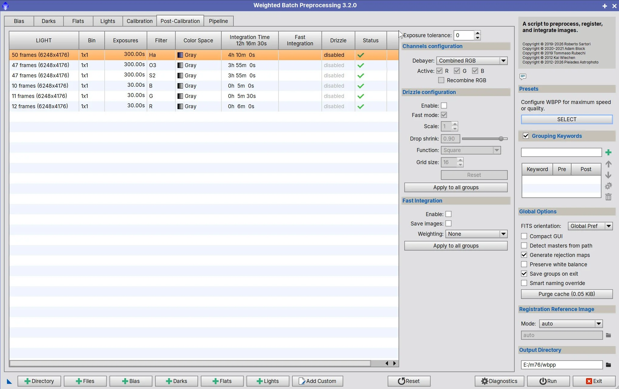
WBPP Post Calibration View
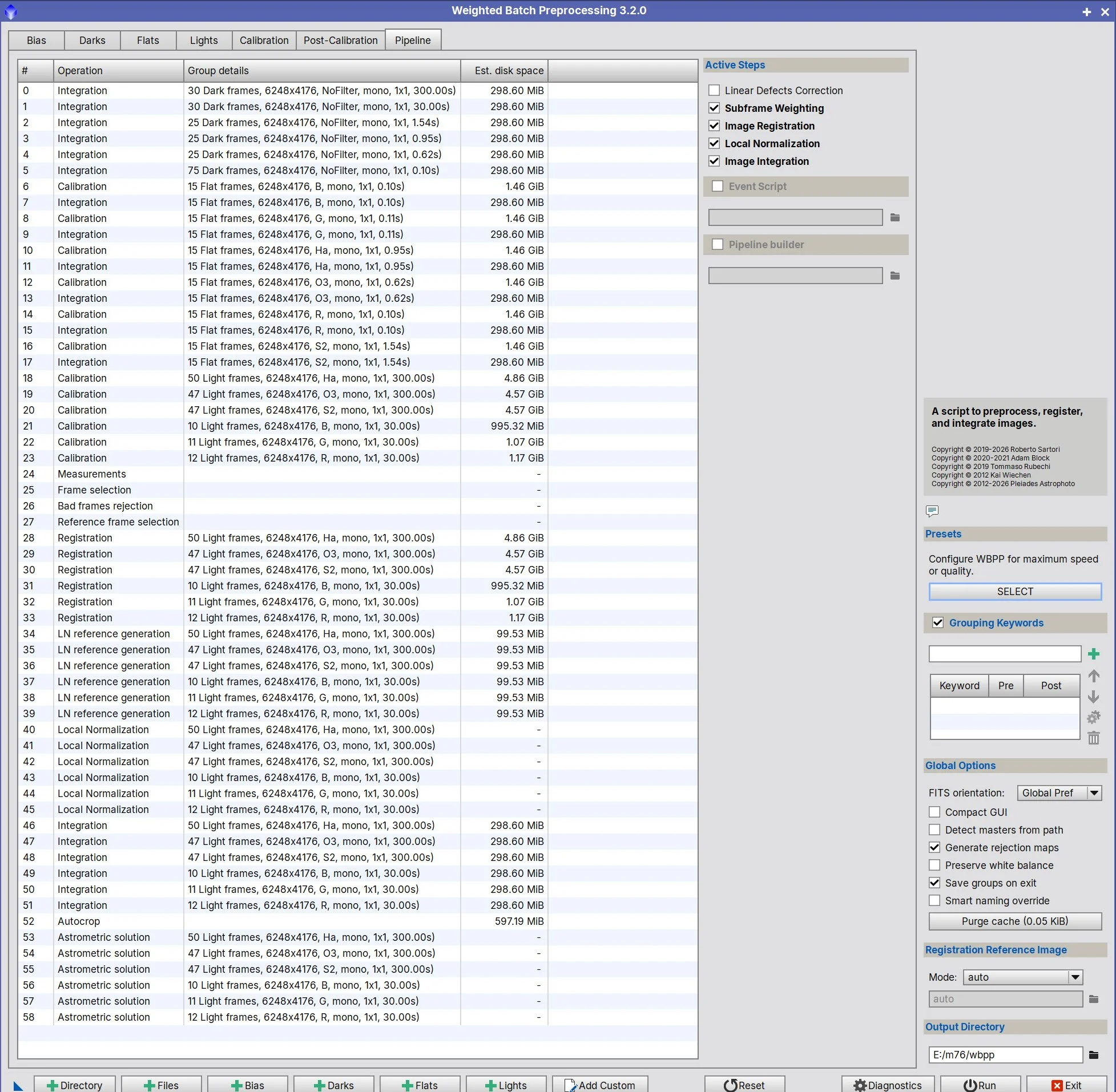
WBPP Pipeline View
3. Load Master Images and Create Color Images
Load all master images and rename them.
Using ChannelCombination, create the master SHO and RGB color images using the following mapping:
R = SII, G = Ha, B = OIII
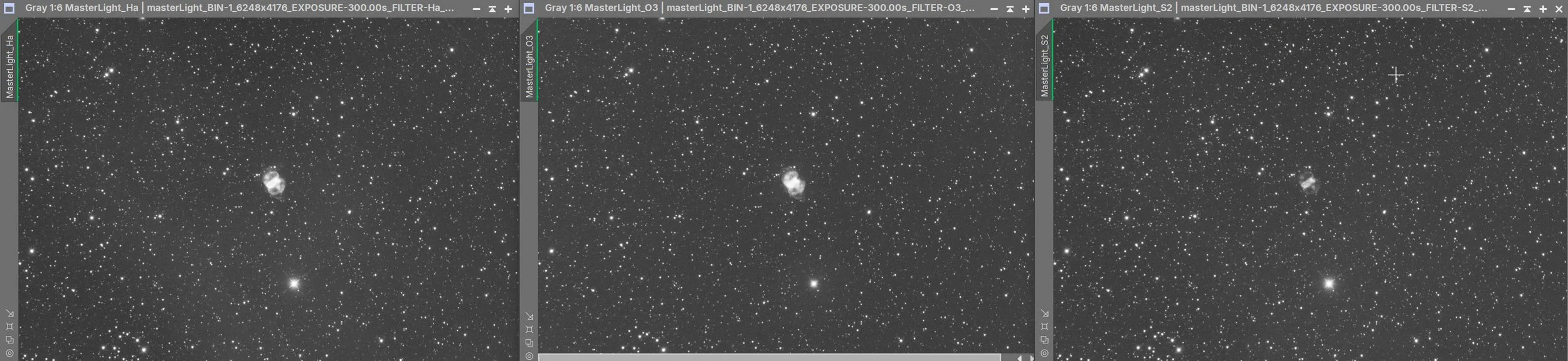
Master Ha, OIII, and SII Images
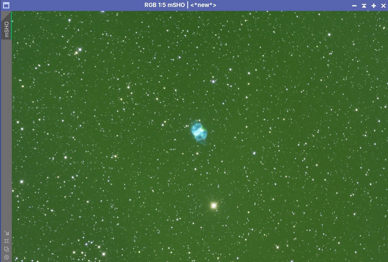
Master SHO image.
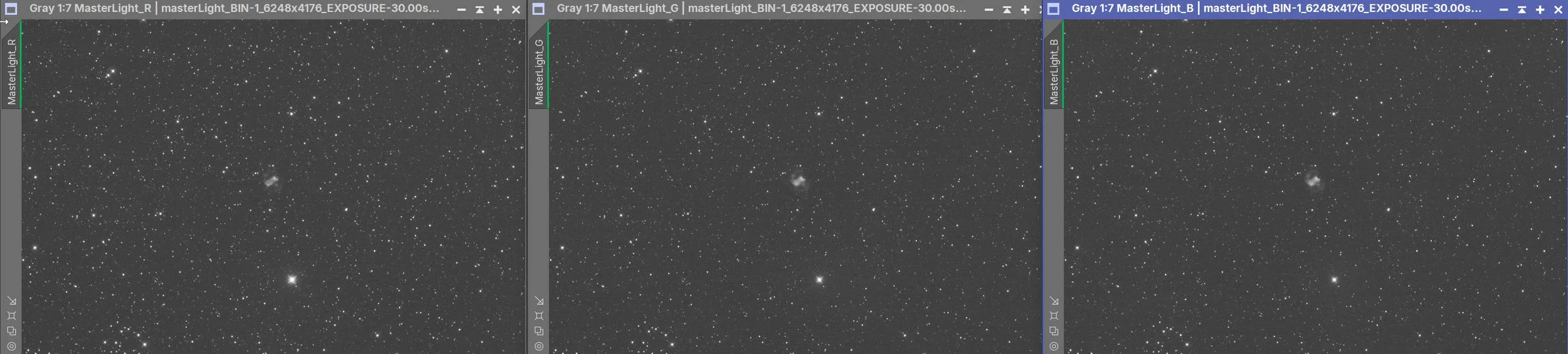
Master R, G, and B images
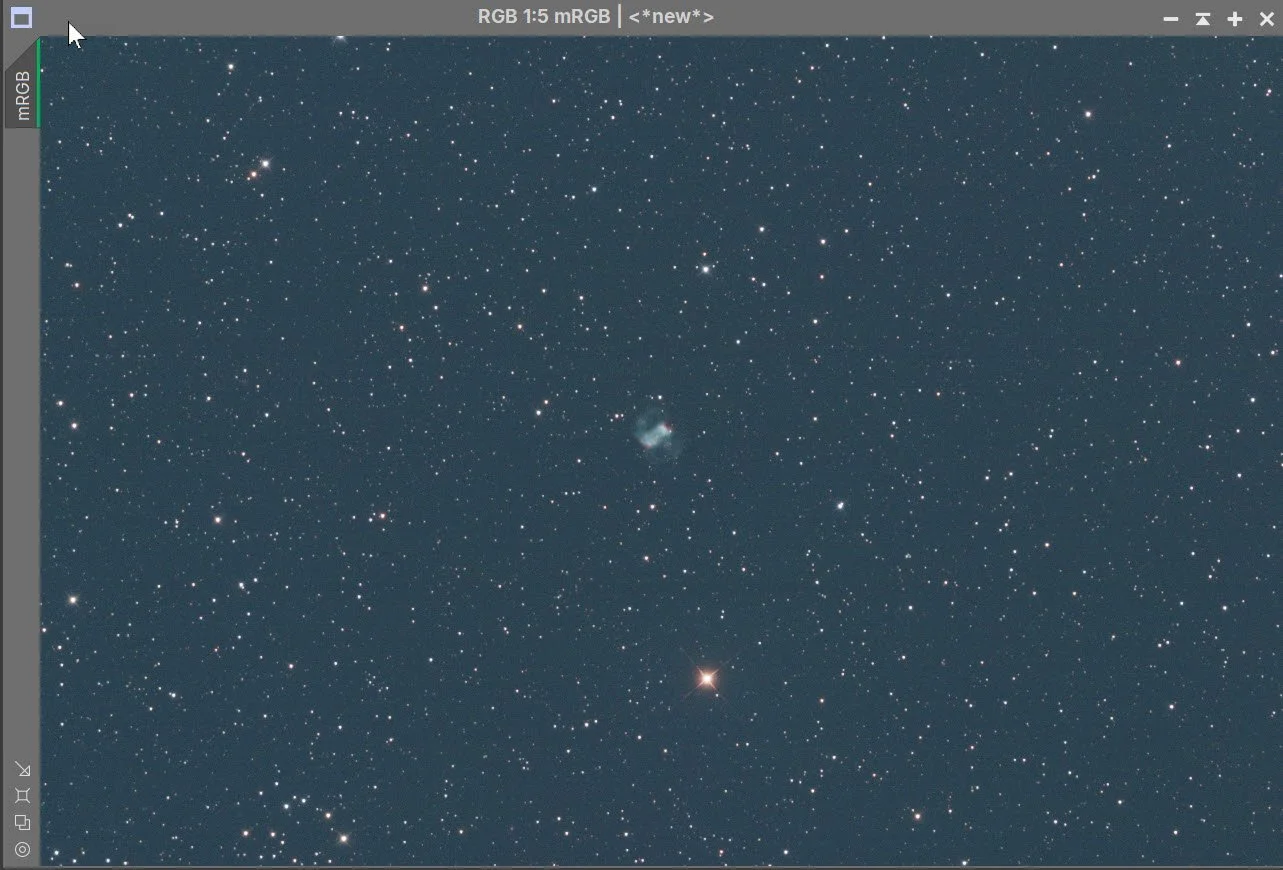
Master RGB color image.
4. Initial Processing of Linear SHO data
DBE was run on the image. Choose a sampling plan that avoids the nebula (see below)
One unexpected problem with this dataset was the distinctly triangular appearance of many stars. I initially attempted to measure the stellar profiles using PFSImage, but the distorted shapes prevented reliable measurements. Consequently, I had to determine the BlurXTerminator settings experimentally. The Correct Only operation was particularly effective at restoring more circular star profiles, and a subsequent full BXT pass provided additional refinement.
Run BXT - correct only. This did an amazing job repairing the stars!
Run full BXT, using settings determined through experimentation.
Run NXT V3 - see params from snapshot below.
Run SXT and remove stars - we are not going to use the narrowband stars, so no need to save them.
DBE Sampling Plan for the SHO image (click to enlarge)
DBE SHO Before Image (click to enlarge)
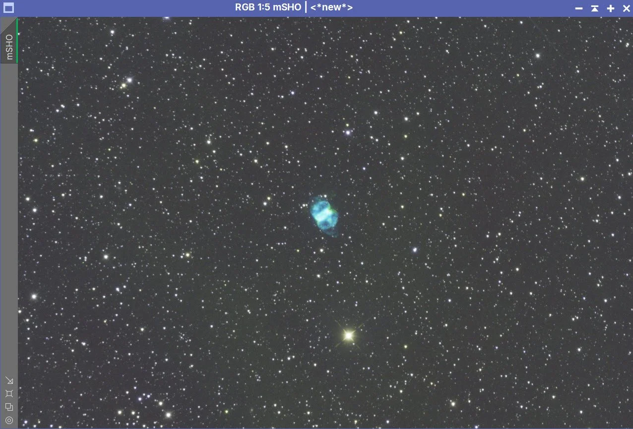
DBE SHO After Image (click to enlarge)
DBE SHO Background Image (click to enlarge)
BXT Settings Used. (click to enlarge)
NXT Panel used. (click to enlarge)
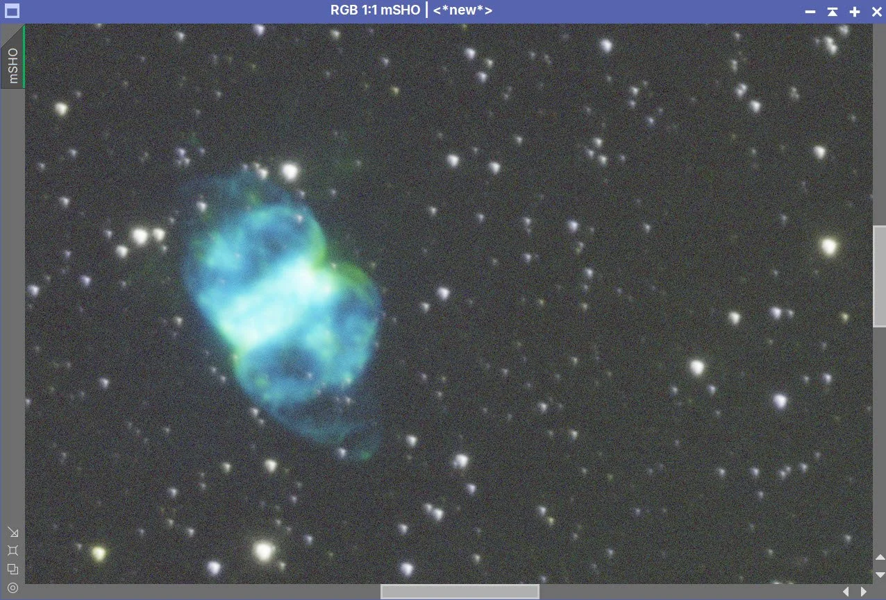
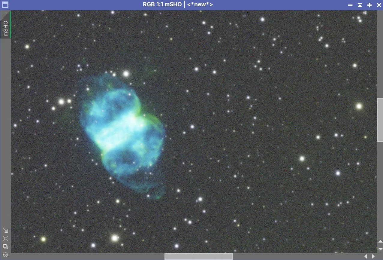
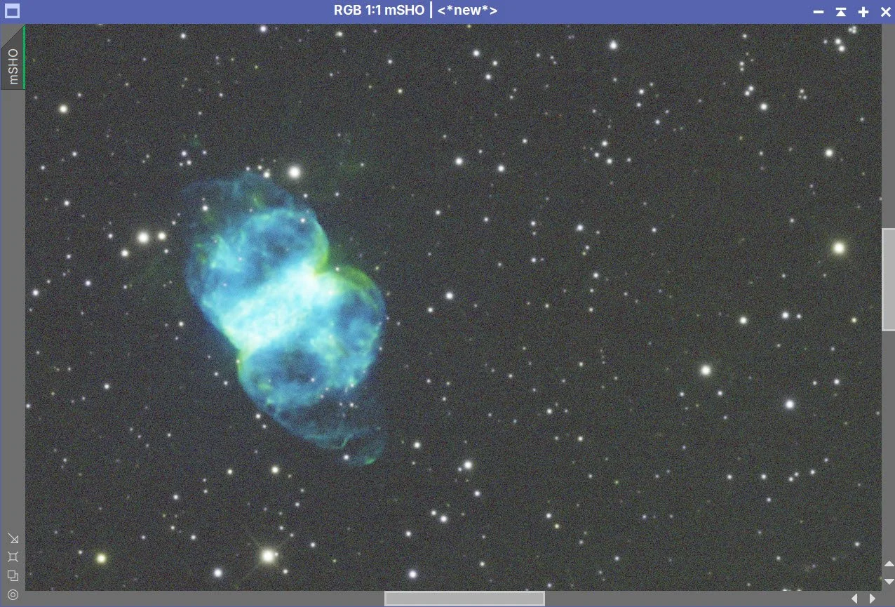
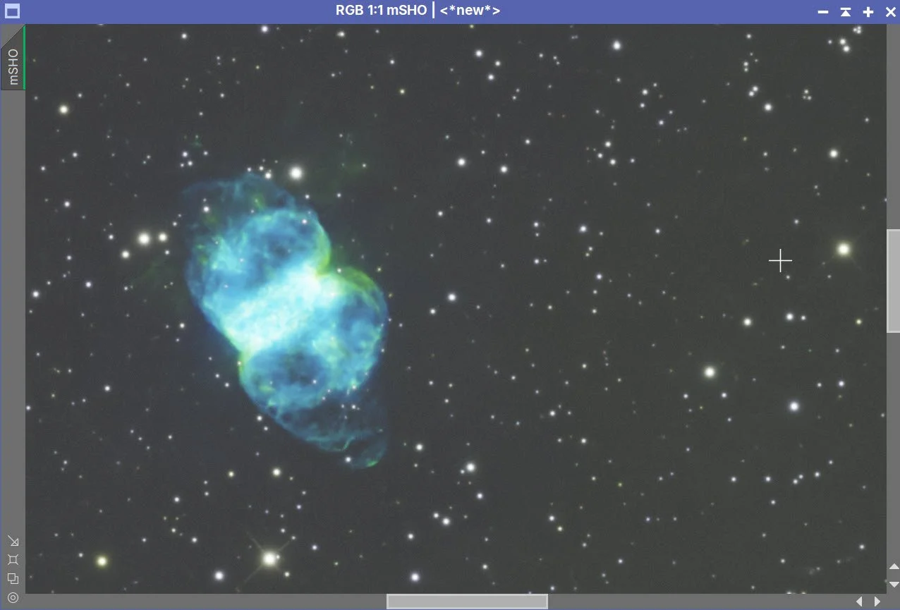
Master SHO Before BXT Correct Only, After BXT Correct Only, After BXT Full, After NXT
Master SHO Image (click to enlarge)
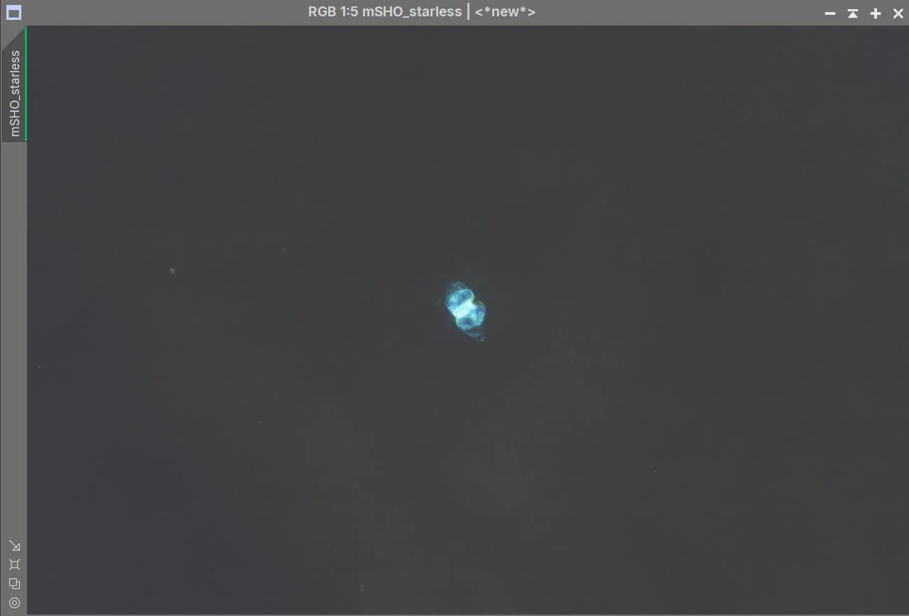
SHO Starless Image.
5. Process the Linear RGB Data
Run DBE on the linear RGB image. Use subtraction for the correction method. Choose a sampling plan that avoids the nebula (see below)
Select a preview rectangle that samples the background sky, and then set up and run SPCC.
Use the Ideal curve
Use ZWO R, G, & B filter curves
Run BXT in Correct Only Mode - this did a great job in correcting the triangular star problem.
Run the Full BXT with terms derived via experimentation.
Apply NoiseXTerminator to the corrected linear RGB image before using StarXTerminator to extract the stars.
Run SXT and don’t save the RGB starless image - we are not going to use that one.
Master RGB DBE Sampling Plan (click to enlarge)
Before DBE (click to enlarge)
Master RGB after DBE (click to enlarge)
Master RGB Background subtracted (click to enlarge)
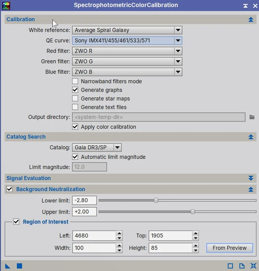
SPCC Panel settings.
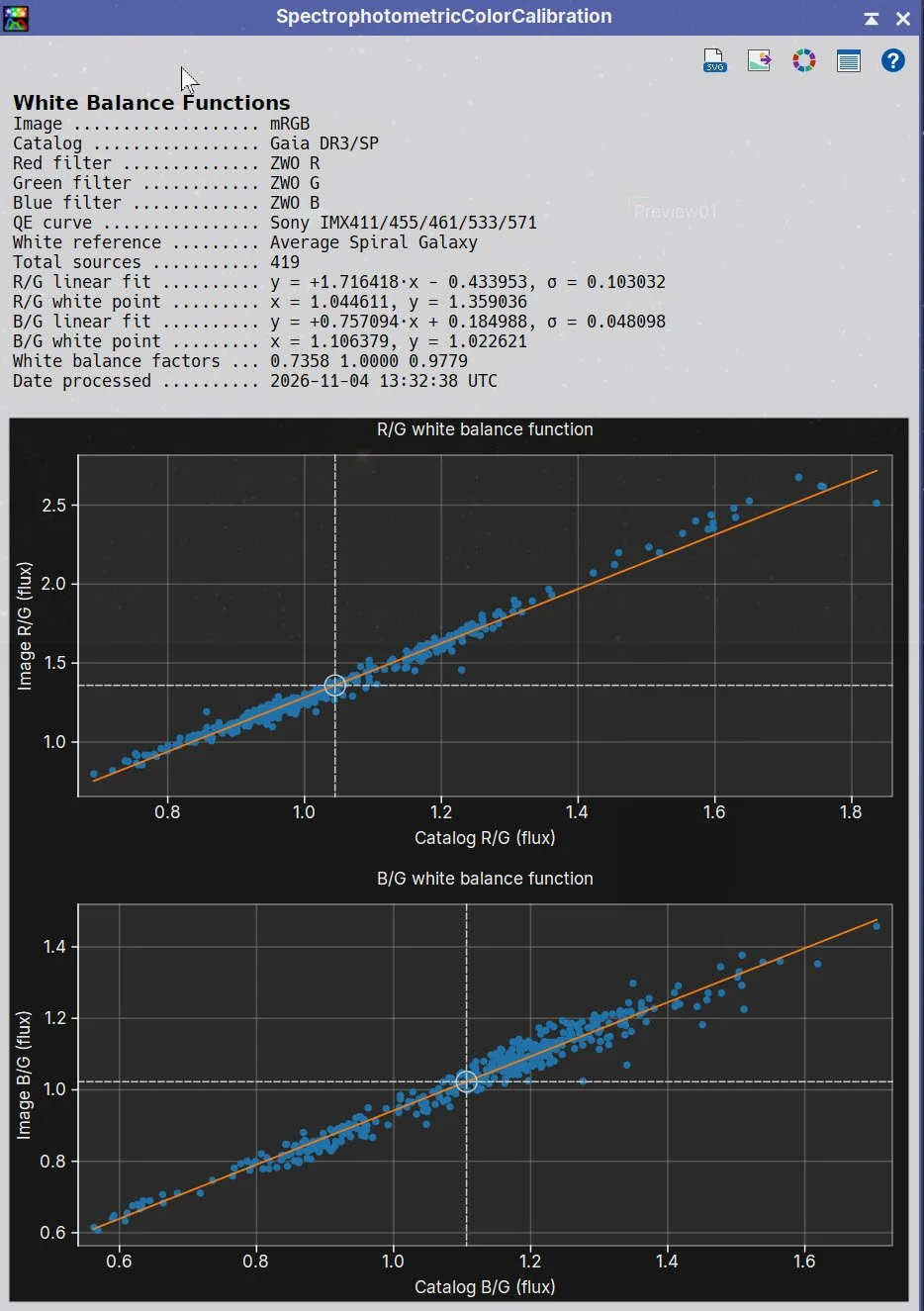
SPCC Regression Results.
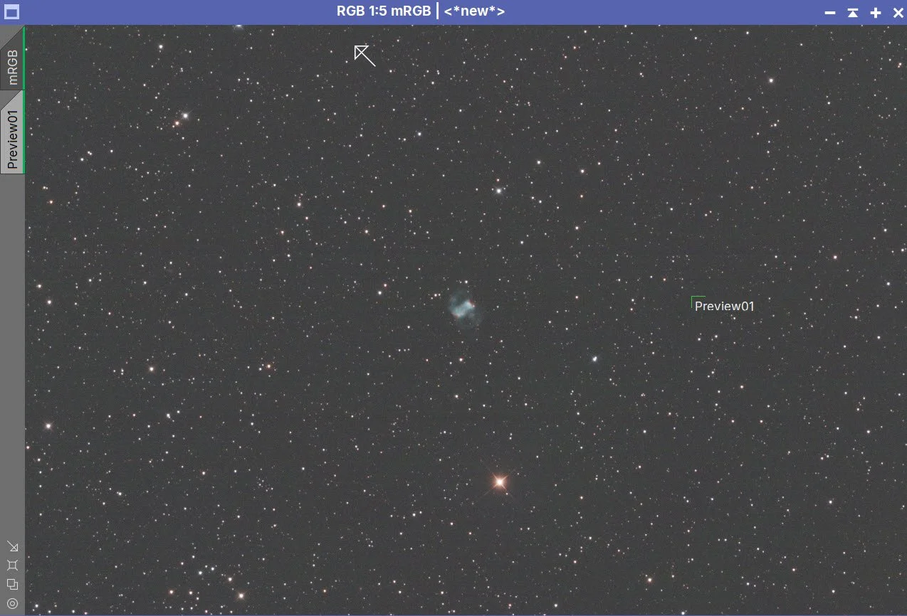
Before SPCC (click to enlarge)
After SPCC (click to enlarge)
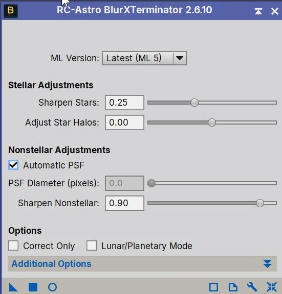
Params used for BXT
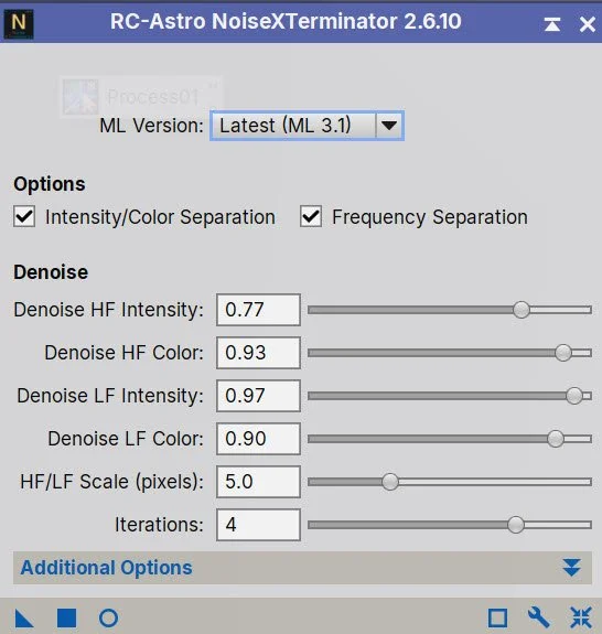
Params used for NXT
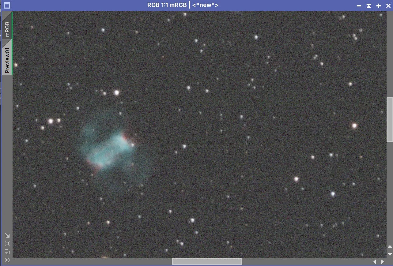
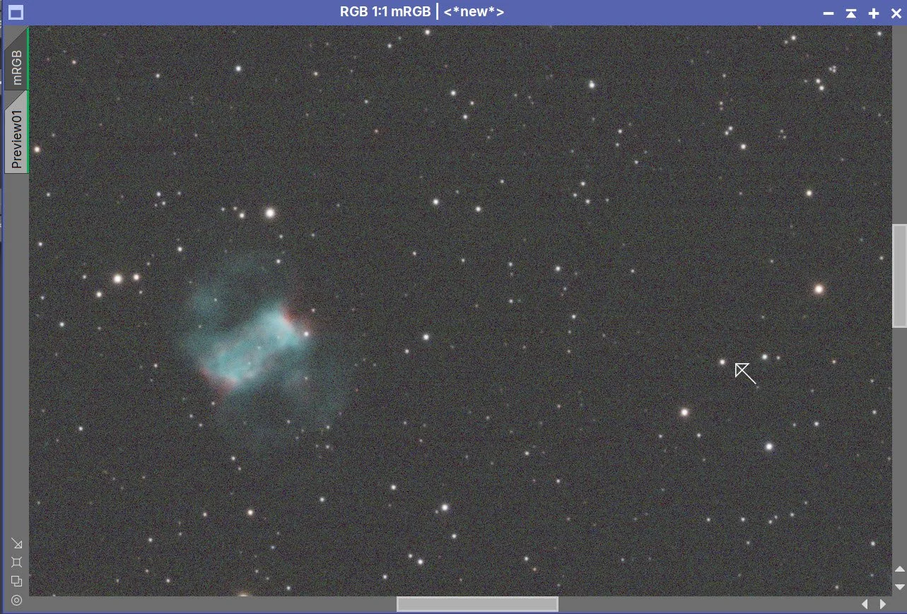
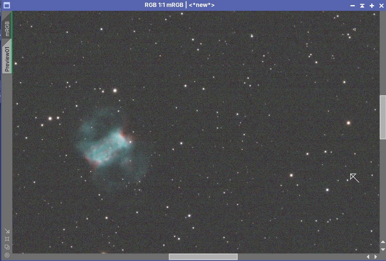
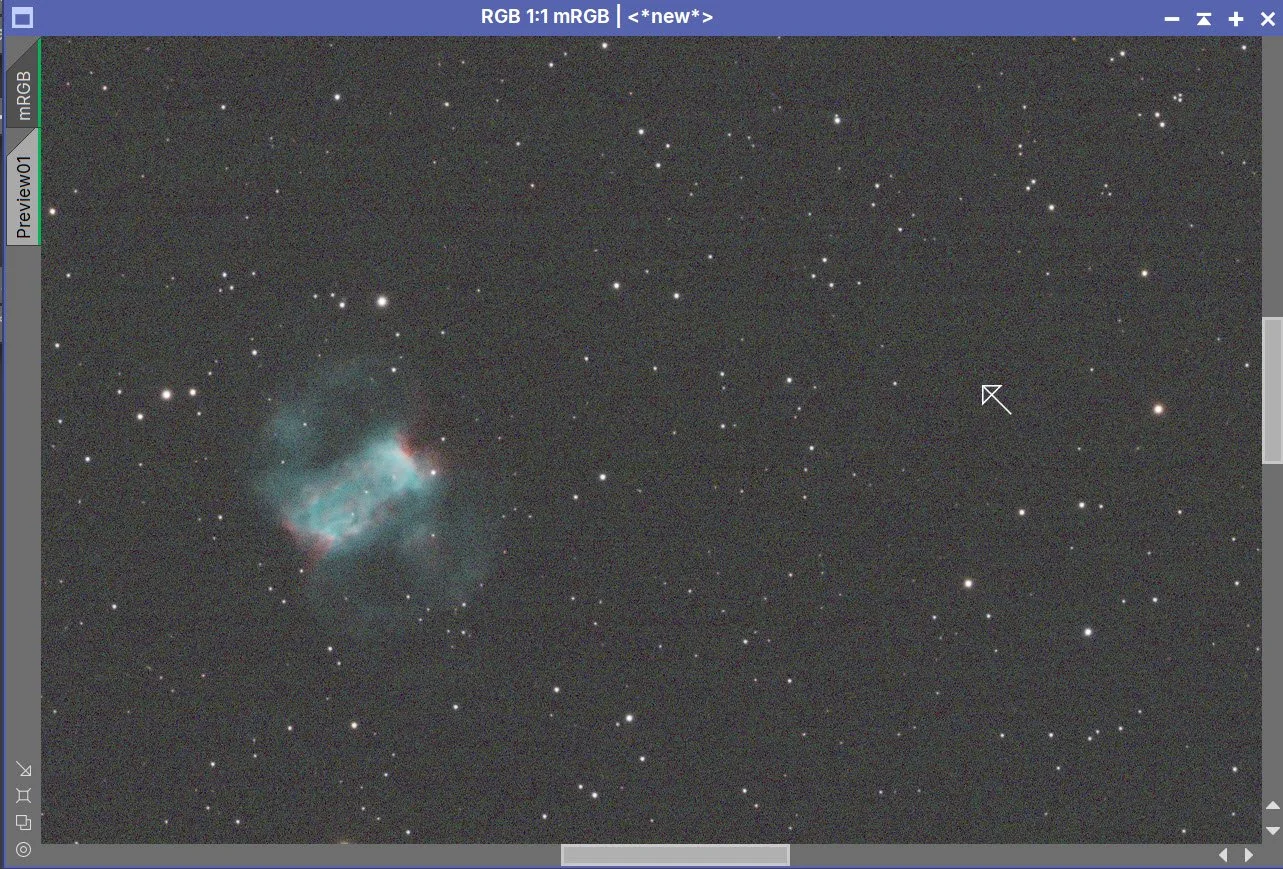
Master SHO Before BXT Correct Only, After BXT Correct Only, After BXT Full, After NXT
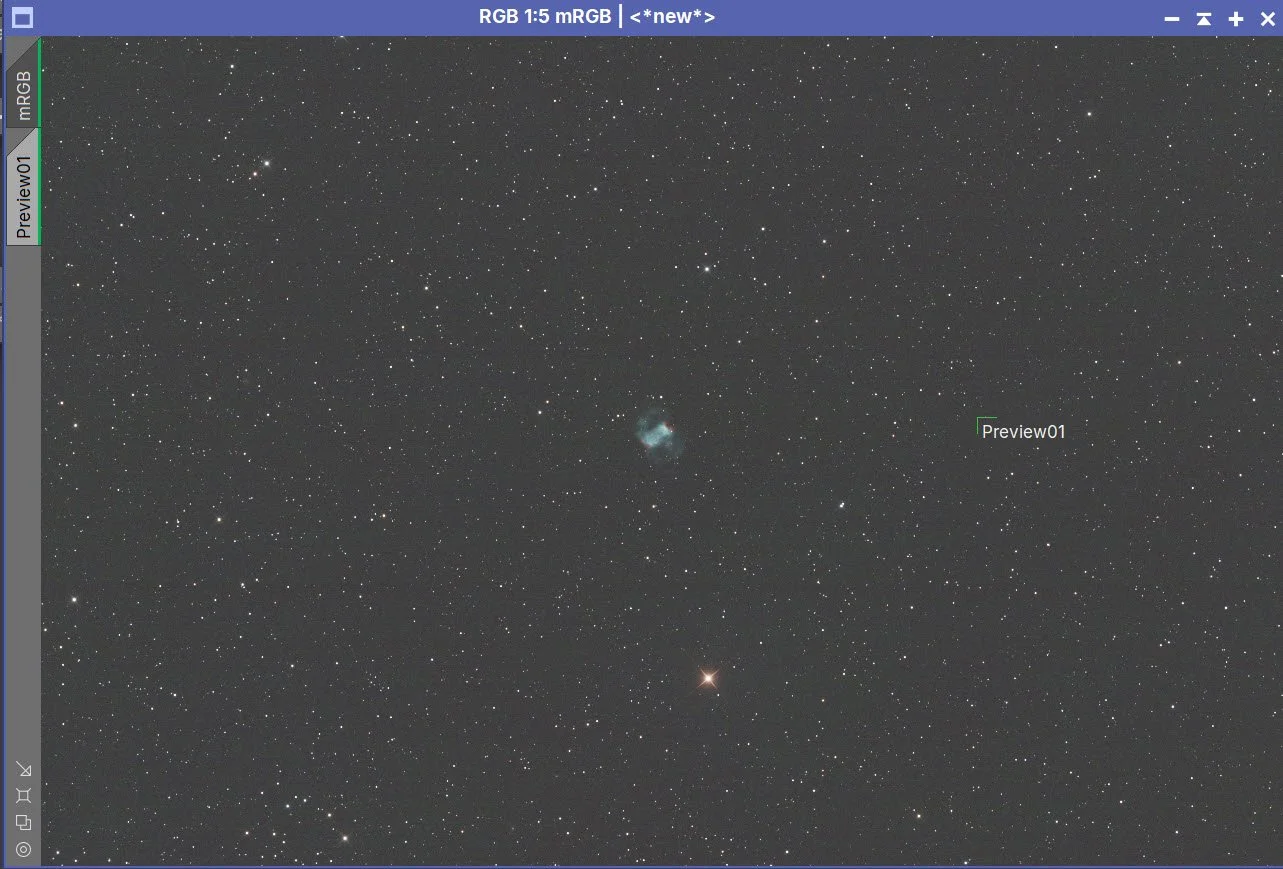
Final RGB Image.
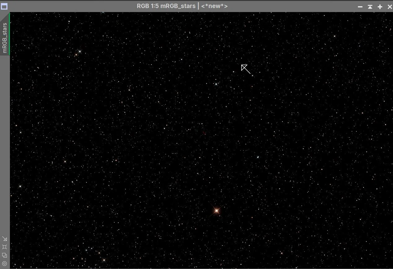
RGB Stars image after SXT.
6. Retain Linear RGB Stars for Astro Star Lab
I no longer convert the RGB stars to a nonlinear form here as I used to. Instead, I leave them alone until the nonlinear starless image processing is complete, then use my new prototype Astro Star Lab to stretch the image, preview the stars against the starless backdrop, and create the final composite image.
7. Take SHO Starless Image Nonlinear
Use the STF→HT method to take the SHO starless image nonlinear.
Nonlinear SHO image
8. Process the Nonlinear SHO Starless Image
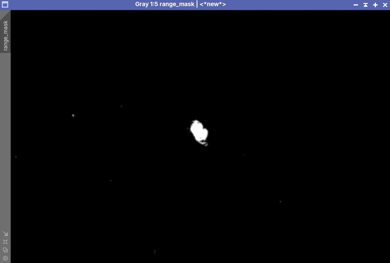
Create a RangeMask using the SelectRange process. This mask will be used later for selective processing, including protecting the bright central nebula while enhancing faint outer emissions and adjusting the surrounding background.
Use the SelectRange Process with parameters shown below.
Now we can start processing the image.
First, I want to recover some compressed tones in the central portion of the nebula using my prototype tool, Astro Tone Recovery. Normally I would use HDRMT for this, but my tool makes it a bit easier to do the same thing. The screenshot below shows the parameters used.
Just a small amount of recovery
And a boost of local detail.
Apply CT to set the basic tone scale and color saturation
The initial SHO image had an undesirable green cast. I first applied SCNR Green at a strength of 0.85 to reduce the green component. I then inverted the image, which transformed magenta regions into green, and applied SCNR Green again at the same strength. Finally, I inverted the image back to its original orientation. This reduced unwanted green and excessive magenta while giving more control over the final color balance:
Apply SCNR for Green at 0.85. This reduced the overall green balance
Then invert the image, which converts magenta regions to green.
Apply SCNR for Green at 0.85 again.
Invert the image - now we should have eliminated the SHO green issue.
Apply another CT to tweak the tone scale and bring up the color saturation a bit.
I still see more green than I like, so I am going to do one final SCNR run
Follow this with a CT for a final tweak.
Now I want to work on the contrast with ACE:
Use the lasso to just select the nebula
Add a tiny amount of Texture (it’s very easy to go too far on this)
Add a touch of Clarity
Now do an MLT sharpening operation - see the params used below.
Now use ACM to finalize the color position. If you push the saturation here, colors block up quickly, so I am using a light touch.
Export the image to Photoshop using a 16-bit unsigned TIFF for some light polishing.
The nebula is looking good, but the faint nebulosity around it is not very apparent. So I am using ExponentialTransformation to bring this up. I am using the inverse of the RangeMask to protect the nebula.
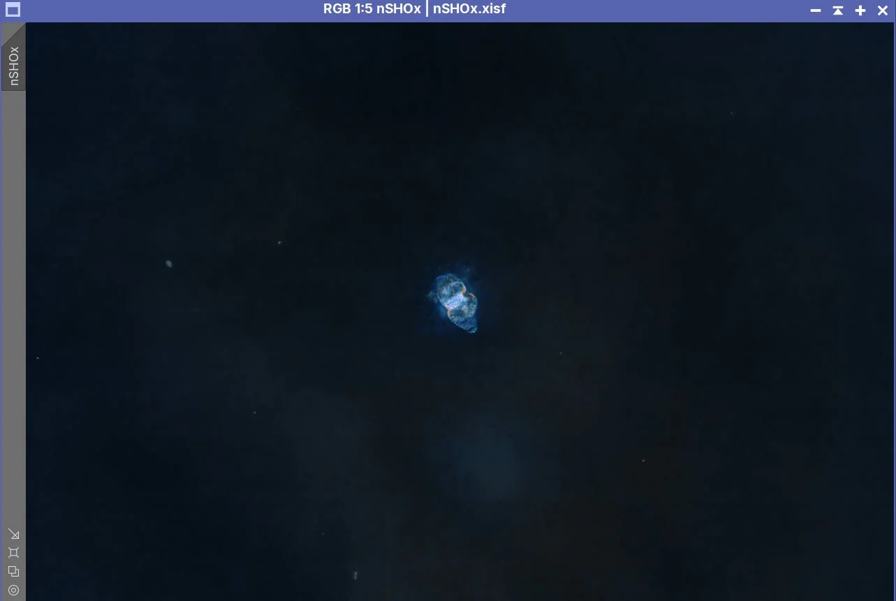
This lightens the background too much, so I am using CT to darken it - again using the inverted of the RangeMask.
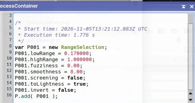
Parameters used to create the RangeMask.
\
Initial SHO Image (Click to enlarge)
Astro Tone Recovery before changes made. (click to enlarge)
After Adjustments (click to enlarge).
After CT (click to enlarge)
Invert the image (click to enlarge)
Another Invert (click to enlarge)
Another SCNR Green at 0.85 applied to handle some of the residual green. (click to enlarge)
NXT parameters used (click to enlarge)
ACE showing the selected nebular region with Clarity adjustment applied (click to enlarge)
After ACE (click to enlarge)
After MLT Sharpening (click to enlarge)
After ACM (click to enlarge)
After ExponentialTransformation with the inverted of the RangeMask (click to enlarge)
After Astro Tone Recovery. (click to enlarge)
After SCNR Green at 0.85 (click to enlarge)
Run SCNR Green at 0.85 (click to enlarge)
Another CT (click to enlarge)
Yet another CT (click to enlarge)
After NXT (click to enlarge)
now with some texture added (click to enlarge)
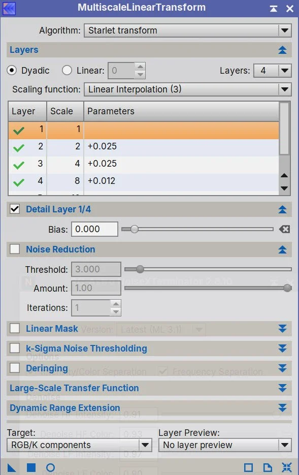
MLT Params Used (click to enlarge)
Use ACM to establish the final color position. (click to enlarge)
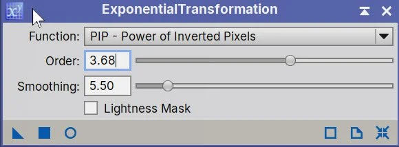
Parameters used.
After A final CT with the inverted RangeMask (click to enlarge)
9. Add the Stars Back In
Here, I am using my Prototype Astro Star Lab script. I let the app do the initial stretch, then added the starless image to get the final effect. I used the preference sliders to tweak things. I brought up the star presence a bit and boosted the star color.
During the final star integration, I noticed what appeared to be a faint dark halo surrounding the brightest star. Using Astro Star Lab's inspection tools, I compared the star with the corresponding area of the starless image. The starless background showed no obvious defect, suggesting that the halo was associated with the star rendering or recombination rather than the background image itself.
This prompted me to add two new correction options to Astro Star Lab: localized background-blemish repair and a background-lift adjustment. In this case, a small increase in local background brightness reduced the apparent halo and created a more natural transition between the star and the surrounding sky.
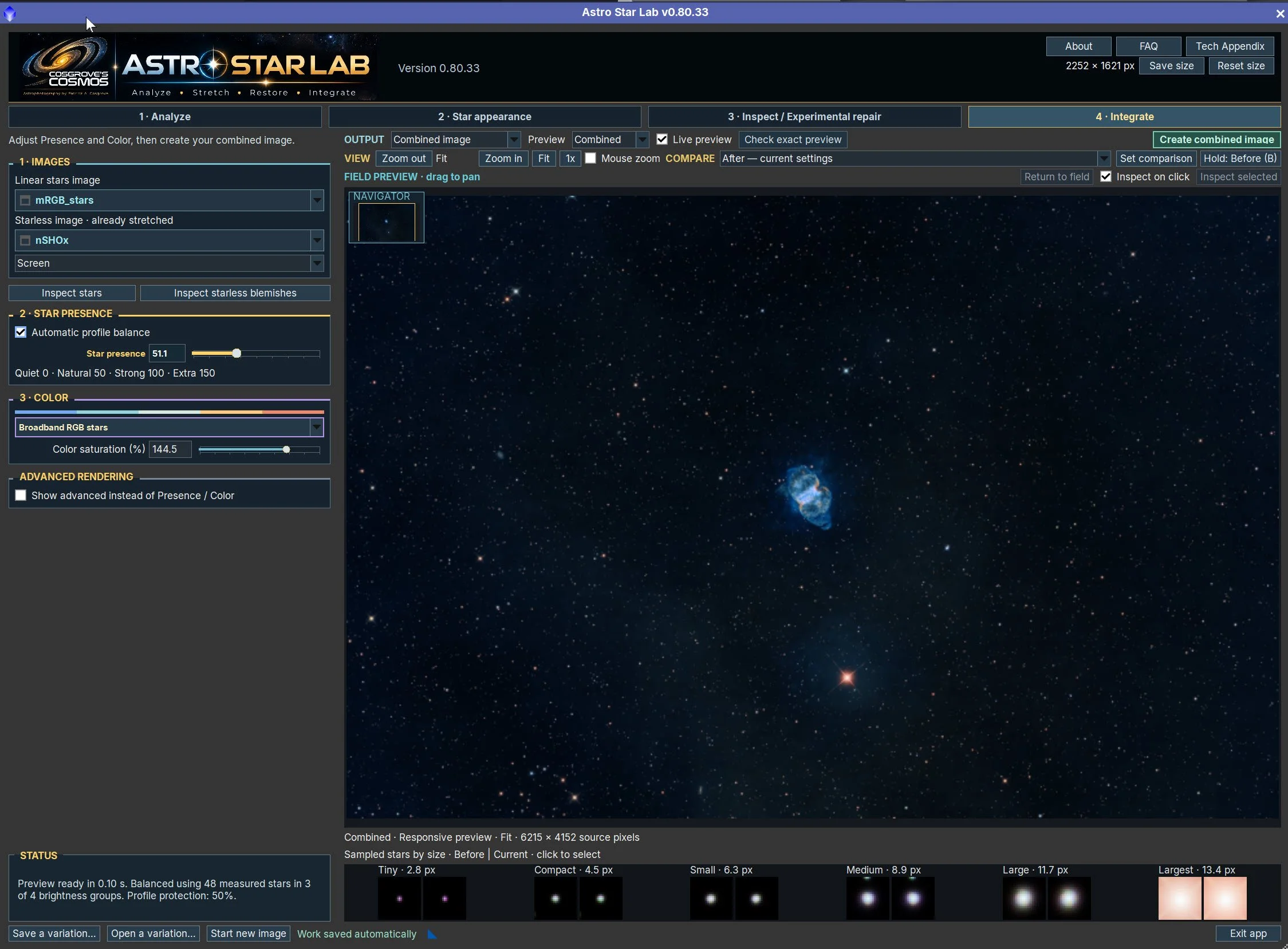
My final setting for the star stretch and rendering.
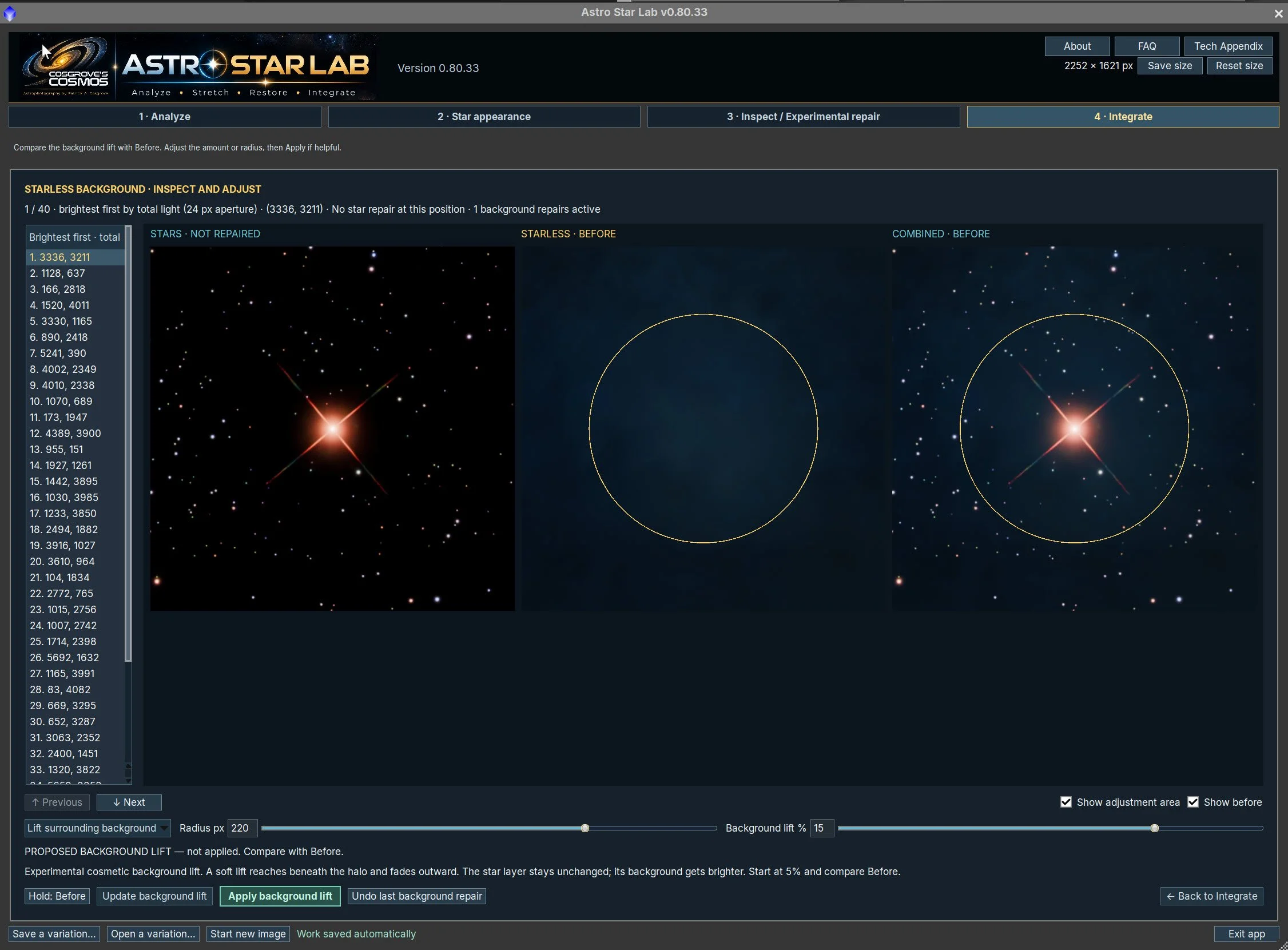
Examining the brightest star. The starless background looked fine. So I used a tool I added that allows for lifting the background slightly to counteract this.
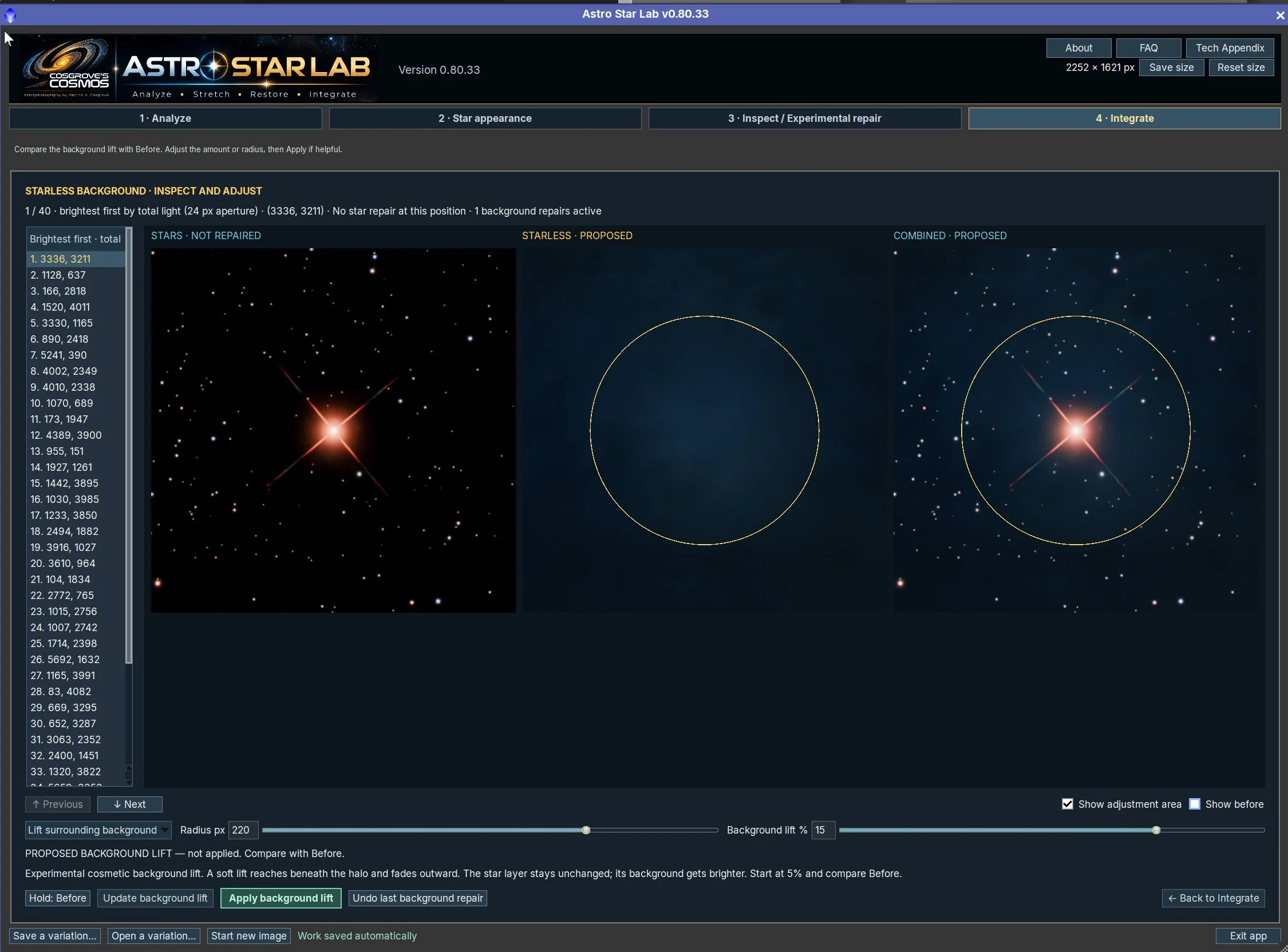
I used the background lift to brighten the background a wee bit and I think this looks better.
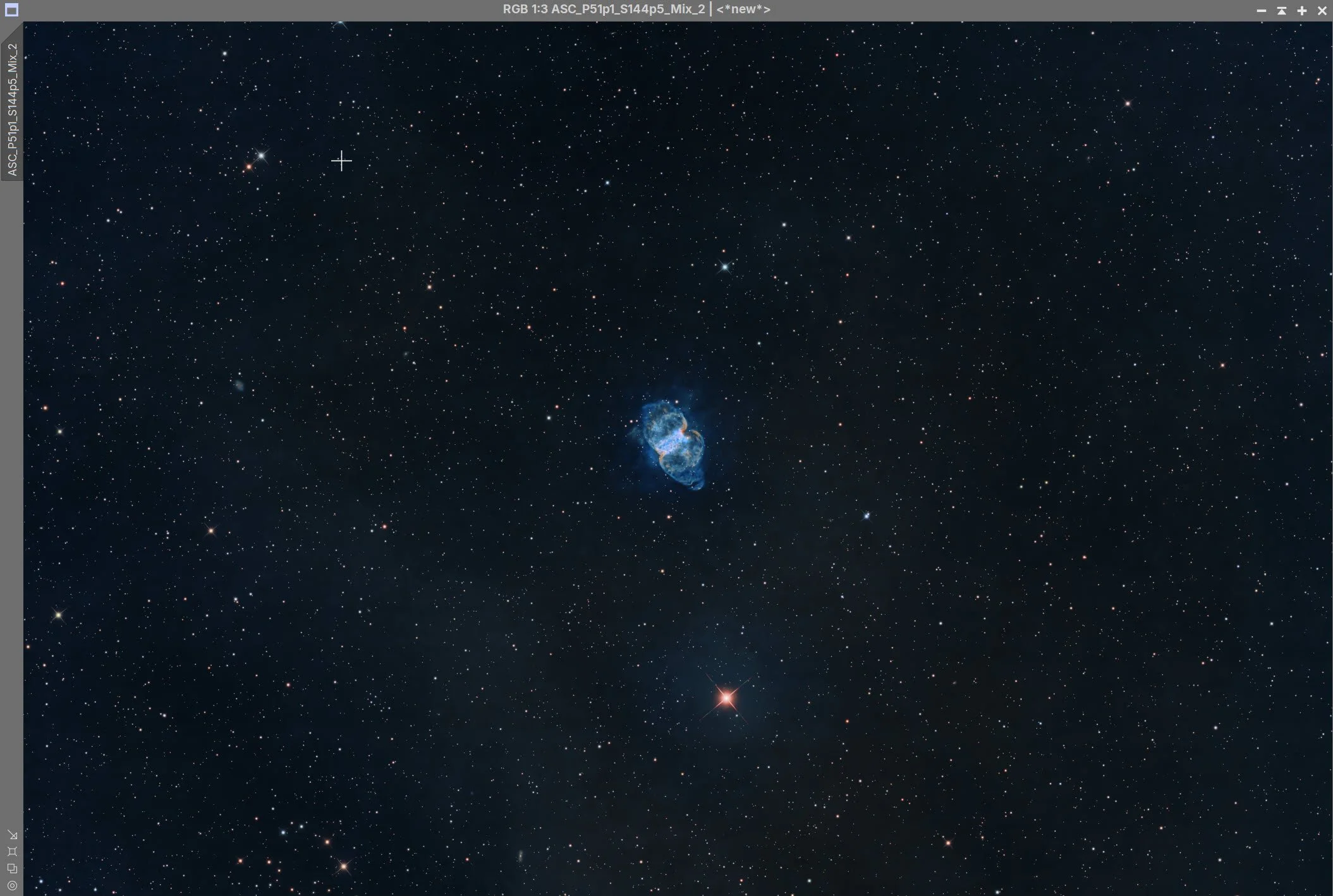
The image - Back with the stars!
10. Export the Image to Photoshop for Polishing
Save the image as a 16-bit unsigned TIFF and move it to Photoshop
My first step was to determine the right crop for this image. I did not want to go too far, and I ended up with the first image
Added watermarks
Export clear, watermarked, and web-sized JPEGs.
11. The Final Image!
Final Thoughts
This project presented several unusual processing challenges. Cloud interference substantially reduced the usable RGB data, while the distinctly triangular star profiles required more corrective work than usual. Fortunately, BlurXTerminator proved remarkably effective in restoring the star shapes, and the surviving RGB exposures were sufficient to produce a satisfactory natural-color star field.
The project also provided an opportunity to use and further develop two of my experimental PixInsight tools: Astro Tone Recovery and Astro Star Lab. Both contributed to the final image, particularly in recovering central nebular detail and achieving a controlled, natural-looking star rendering.
The final result reveals the intricate central structure of M76 together with its much fainter outer lobes. Despite the acquisition and processing challenges, I am pleased with the level of detail and the balance achieved between the bright nebula, faint surrounding emission, and background stars.
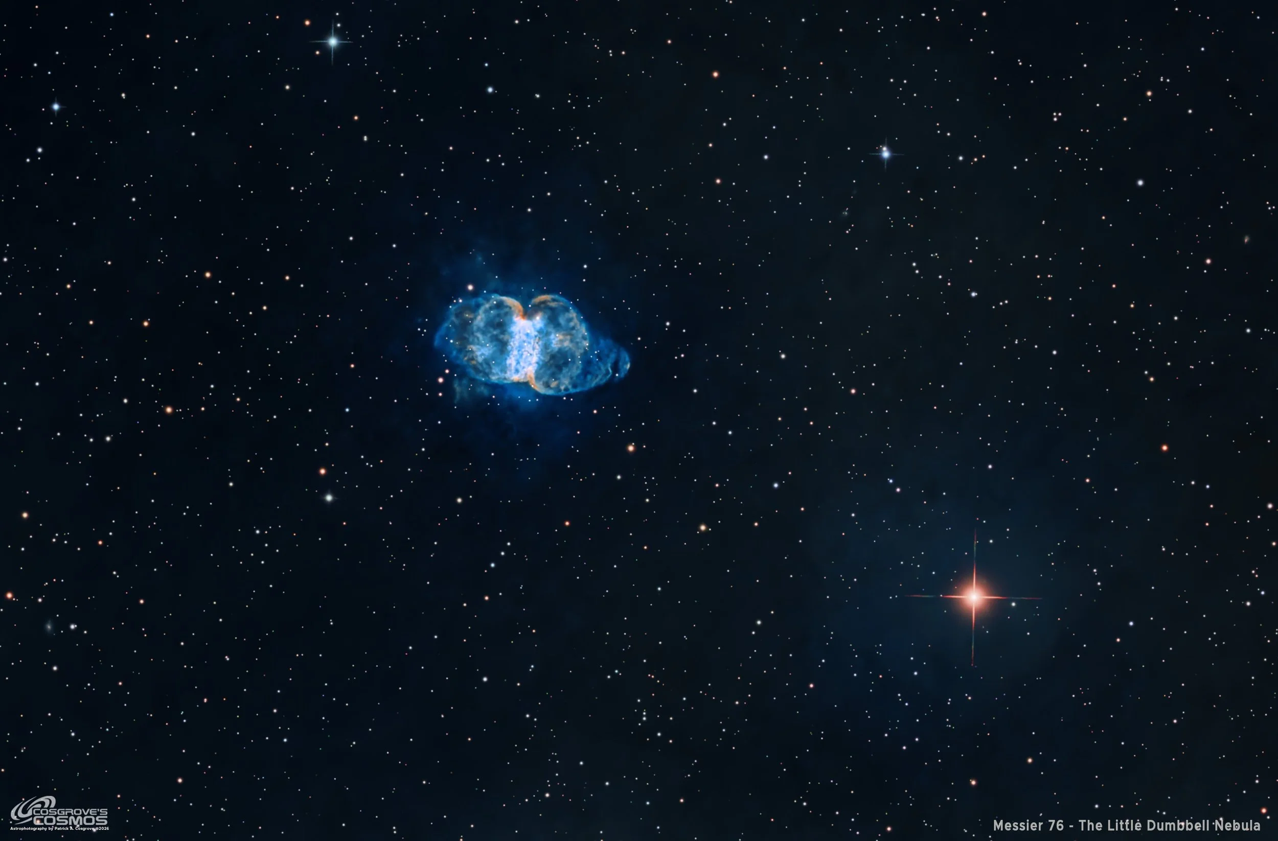
The Final Image
Back to the Main Messier 76 - 2026 Page
Alternatively, you can use the back arrow to return to the Main M76 page, or you can use the menu at the top of the page to continue your navigation.
Thanks,
Pat