
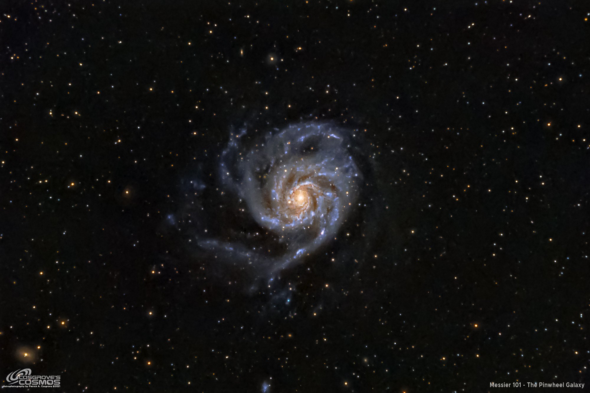
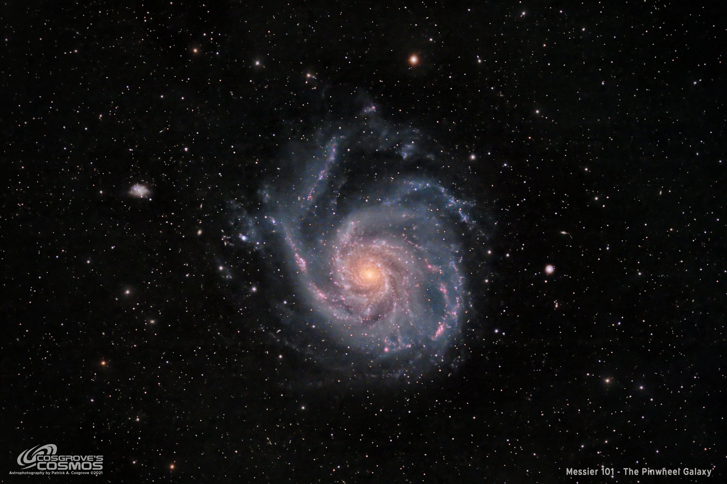
M101 - The Pinwheel Galaxy in LHaRGB (11 hours)- a third attempt!
Date: May 11, 2022
Cosgrove’s Cosmos Catalog ➤#0098

Awarded “Explore” Status on Flickr on May 12, 2022!

This is my third attempt at M101 - while I am happier with this image compared to my previous two attempts, it still offered a series of processing challenges. (click for high resolution version of the image via Astrobin.com)
Table of Contents Show (Click on lines to navigate)
About the Target
A little about M101- from Wikipedia:
“The Pinwheel Galaxy (also known as Messier 101, M101 or NGC 5457) is a face-on spiral galaxy 21 million light-years (6.4 megaparsecs) away from Earth in the constellation Ursa Major. It was discovered by Pierre Méchain in 1781 and was communicated that year to Charles Messier, who verified its position for inclusion in the Messier Catalogue as one of its final entries.
On February 28, 2006, NASA and the European Space Agency released a very detailed image of the Pinwheel Galaxy, which was the largest and most-detailed image of a galaxy by Hubble Space Telescope at the time. The image was composed of 51 individual exposures, plus some extra ground-based photos.
On August 24, 2011, a Type Ia supernova, SN 2011fe, was discovered in M101.”About the Project
The Annotated Image
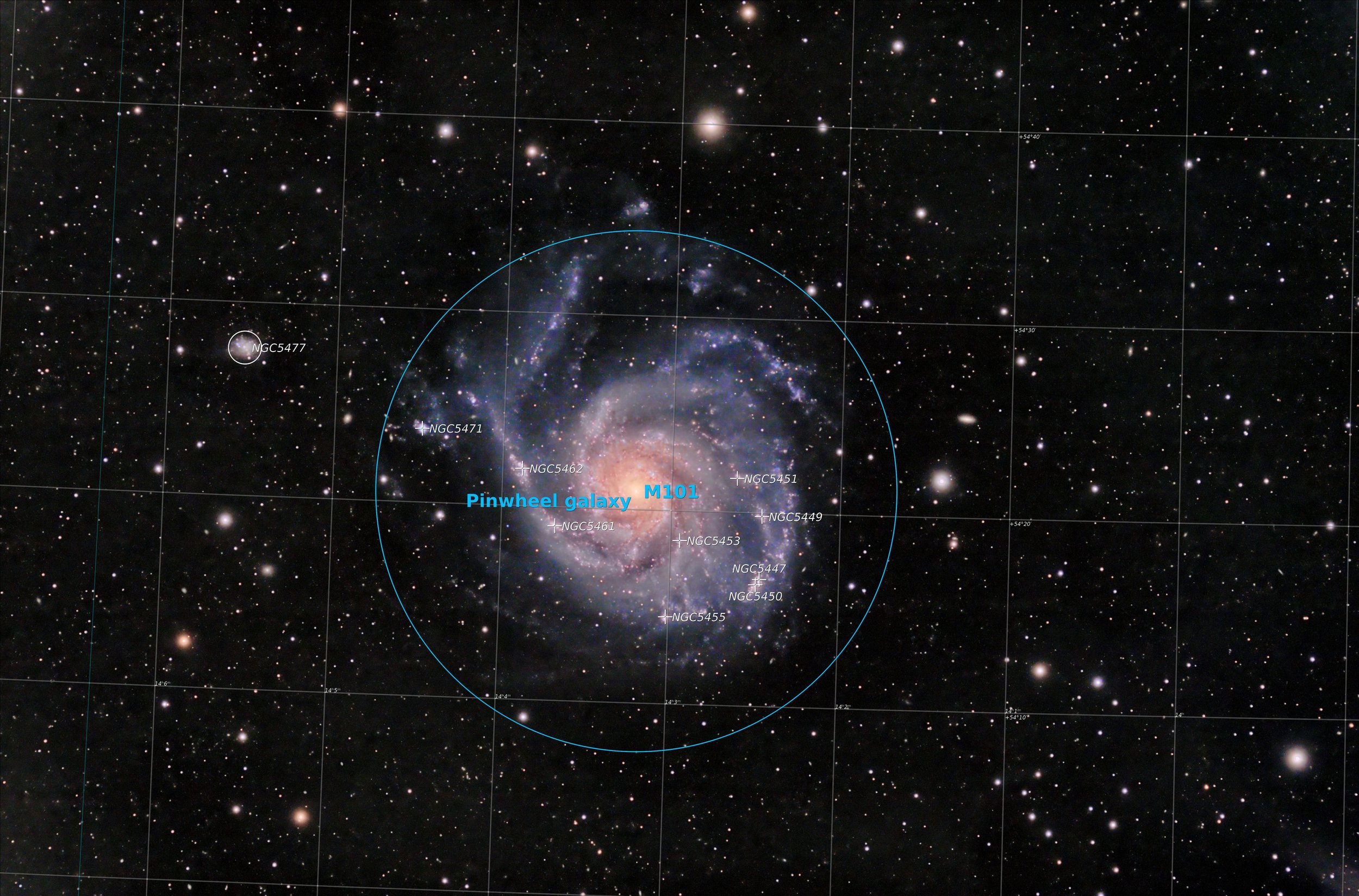
Annotation created with the ImageSolve and AnnotateImage scripts in Pixinsight.
The Location in the Sky
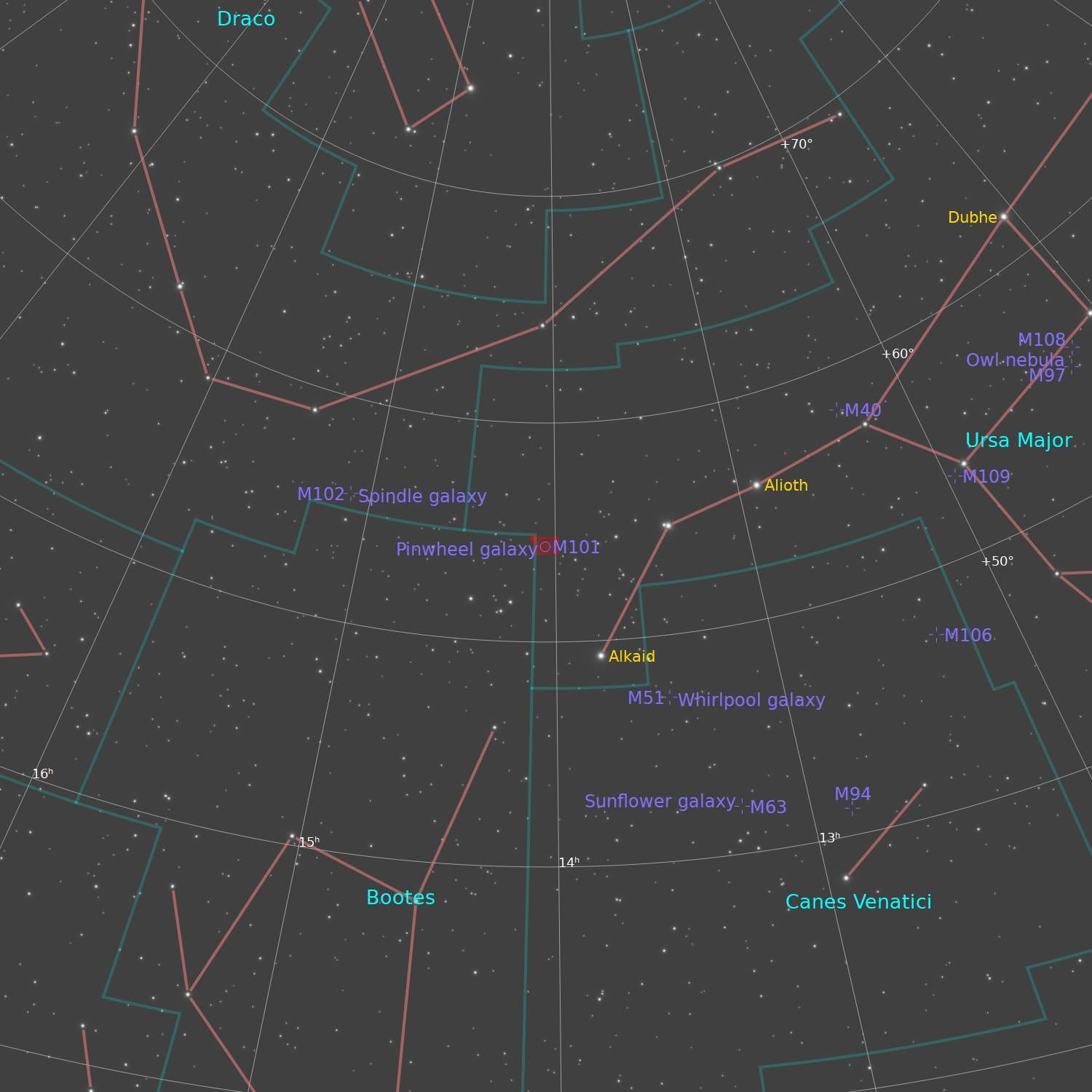
This ap created using the FinderChart process in Pixinsight.
About the Project
Background
Ahhhh….Messier 101! I’ve been here before.
The first time I shot M101 was back in May of 2020. I shot for two hours with an OSC camera and reasonable result for such a short integration time and my relative inexperience back then. You can see the results HERE.
A year later, in May of 2021, I decided to try again. I was now experienced shooting with a mono camera and had another year’s experience under my belt. I was excited to see what I could produce. I captured M101 for 5 nights! ( I know - five clear nights in a row in western New York?) This would have been one of the longest integrations I had ever done. I could not wait, that is until I looked at the data. Over the 5 nights, thin clouds came through and caused me to throw out 1/3 of my subs. OUCH. Then I stacked the data and discovered that I had a horrible problem with pattern noise! This is usually avoided by dithering your exposure - which I thought I was doing. But something went wrong and the rainbow-colored smears of data were hard to fix and I had to beat the processing hard to salvage something from all of that work. The result was pretty bad - as I look at it now, it makes me cringe! That image can be seen HERE.
Another Chance
After the horrible experience of last year, I really wanted to try this again and see if I could do better.
This has been a tough year so far weatherwise. Up until now, I have only had two capture sessions of two hours each. Pretty sad really.
But we finally got a break and it looked like we might have three or maybe four clear nights with no moon starting on 4-28-22. We ended up having only two clear nights. Dan Kuchta was doing some imaging at the same time and collecting data to understand the seeing. According to his work, the seeing on the first night was worse than average. We typically get 2.5-3.0 arcseconds of seeing but on these evenings, we had it as bad as 5.0 at some points. Even still - it was clear and I was able to get two nights of data. Once M101 cleared the trees, I had about 3 hours before it re-entered the tree line. The third evening was a bust weatherwise so I waited to see if I could somehow get one more night in before wrapping up the project. And as luck would have it, I got one more chance to collect data on the night of 5-5-22. It had rained all day long and just started to clear as darkness fell. Humidity was at 100% but it was clear and I went for it.
I ended up collecting a little over 11 hours of LRGB and Ha data collected on my Astro-Physics 130mm f/8.35 scope and my ZWO ASI2600MM-Pro camera.
Camera Sampling
My first image was shot with my first Astro camera - the ASI294MC-Pro. My Second Attempt was shot with my Second Astro Camera and my first Mono camera - the ASI1600MM-Pro. This current image was shot with my newer ASI2600MM-Pro. So without meaning to, I have sampled all of my Astro cameras on this target as well!
Processing Frustrations
I usually enjoy the processing process. However, I did NOT enjoy processing this image. I ended up doing three separate processing runs.
The first time I processed it, I decided to drizzle process the already high res data from the 2600 camera. It took WBPP forever to calibrate the data and the master images were so big that every operation I did on the was slow and cumbersome. I got about halfway through the editing process to discover that Pixinsight was complaining that the hard drive was full! I never had that happen before. I cleaned out what I could but if I wanted to deal with drizzle processing from this camera, I need more disk space! I decided that drizzle processing here was overkill. I deleted everything and started over from scratch - this time with no drizzle processing!
The second time processing this image was going really great. I was making good progress and I was very happy where the image seemed to be going… and then for no particular reason, my power went out and then right back on. Of course, the computer rebooted and I lost over two hours of processing. AHHHHHHH! (I just ordered a UPS for this computer - this will never happen to me again!)
This is the third time I shot M101 and my third time processing the data and now I have a final image.
So - all is good with the world. - right? Well. - not quite.
The good news is that the final image is not half bad. It is better than my first, and way better than my disastrous second image. The bad news is that I am still not that happy with it. I expected better. I ran into two issues that I believe held me back:
The bright stars were very bloated. I think the poor seeing and the humidity of the last night caused the brighter stars to bloat and great larger than desired images. I used several tricks to reduce this bloat, but the stars do not look as good as I would like because of this. Don’t look at the bright stars too close, you won’t like what you see there.
The fainter aspects of the galaxy arms are still not as well defined as I would like. M101 is towards the north for me - and in that direction is the city of Rochester, NY. I think I am fighting the light pollution of the city.
Here is a comparison of my three attempts so far:
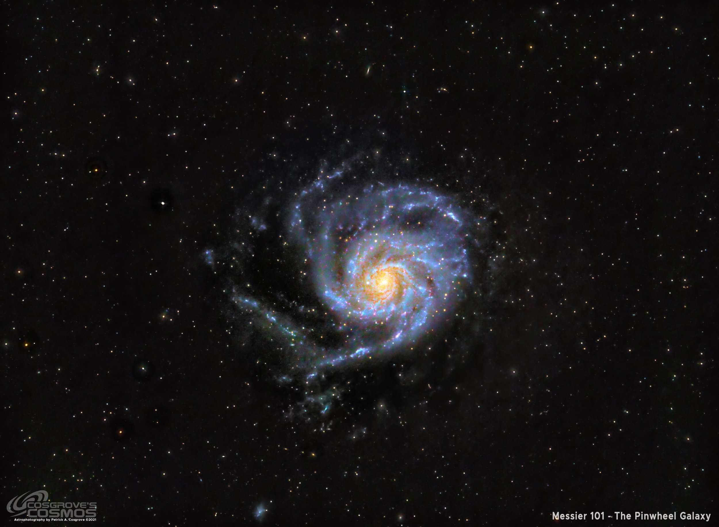
The final version has reasonable color, but is it correct? I did a search on Astrobin, looking at all of the image of M101 that have been named “Top Pick Candidates”. There were as many colors positions as there were images - so I guess this is as good as any.
Please note that there are detail processing notes that can be found at the end of this posting.
More Information
Wikipedia: M101 Entry
Nasa: Hubble Image of M101
Jet Propulsion Labratory: Infrared Image of M101 from the Spritzer Telescope
Capture Details
Light Frames
Data was collected during the Nights of 4-28-22, 4-29-22, and 5-5-22
115 x 90 seconds, bin 1x1 @ -15C, unity gain, ZWO Gen II L Filter
88 x 90 seconds, bin 1x1 @ -15C, unity gain, ZWO Gen II R Filter
88 x 90 seconds, bin 1x1 @ -15C, unity gain, ZWO Gen II G Filter
65 x 90 seconds, bin 1x1 @ -15C, unity gain, ZWO Gen II B Filter
29 x 300 seconds, bin 1x1 @ -15C, unity gain, Astronomiks 6mm Ha filter
Total of 11.3 hours
Cal Frames
30 Dark exposures
30 Flat Darks at appropriate flat exposure times
15 L Flats
15 R Flats
15 G Flats
15 B Flats
Image Processing Detail
(Note this is all mostly based on Pixinsight with some Photoshop polishing at the very end.)
1. Assess all captures with Blink
Light images
Lum: All images looked good. Some star trails that will be handled by ImageIntegration
Red: All images looked good. Some star trails that will be handled by ImageIntegration
Green: All images looked good. Some star trails that will be handled by ImageIntegration
Red: All images looked good. Some star trails that will be handled by ImageIntegration
Ha: 3 images rejected due to cloud coverage.
Flat Frames - look great!
Flat Darks - looks great!
Darks - taken from earlier cal files
2. WBPP Script 2.41
All images - lights, flats, and flat darks loaded into the tool.
The script panel was set up for:
Cosmetic Correction
Automatic Pedestal image handling
Gradient Normalization
Calibration and registration only
The Script ran for several hours - even though it was a 12-core Ryzen system! Handling gradients seems to slow things down!

The WBPP Calibration screen.

The Post Calibration Screen
3.0 Image Integration
Each image was integrated by hand after calibration was done. I noticed that a new method was now available for pixel rejection called Robust Chauvenet Rejection (RCR). I decided to try this out with the Lum image. I ran the integration with this new method and the default parameters as well as ESD, using its default parameters. Reviewing the High Rejection images created for both, I thought that the new method seemed to be doing a better job and decided to use it for this image.
L, R, G, B, and H Images were integrated and the resulting master images were pulled into Pixinsight.

The Image Integration Panel is set up for Robust Chauvenet Rejection.

Now set up for the ESD method of rejection that I often use.

The RCR rejection method seemed to throw out a bit more junk as shown in this High Rejection image for Lum.

Here is the High Rejection result for ESD.
4.0 Dynamic Crop
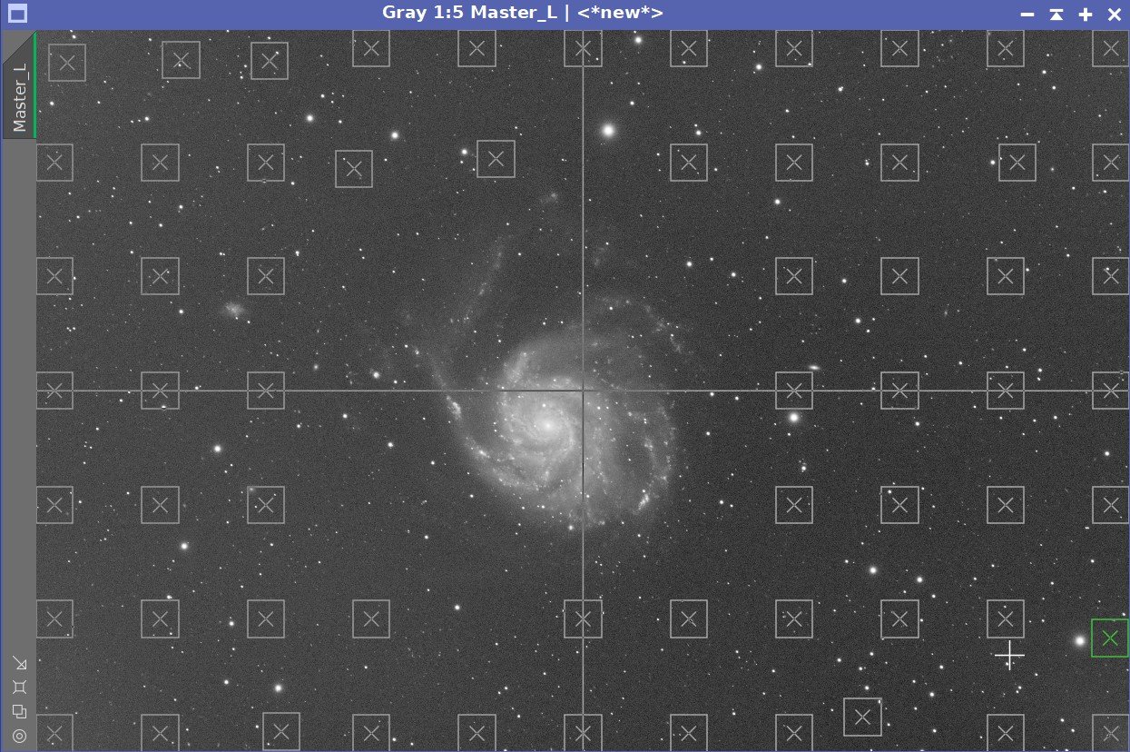
Master Images were imported into Pixinsight, and a common best crop position was used and implemented with DynamicCrop.
5.0 Dynamic Background Extraction
There we some images with residual gradients that had to be dealt with and DBE was used on each.
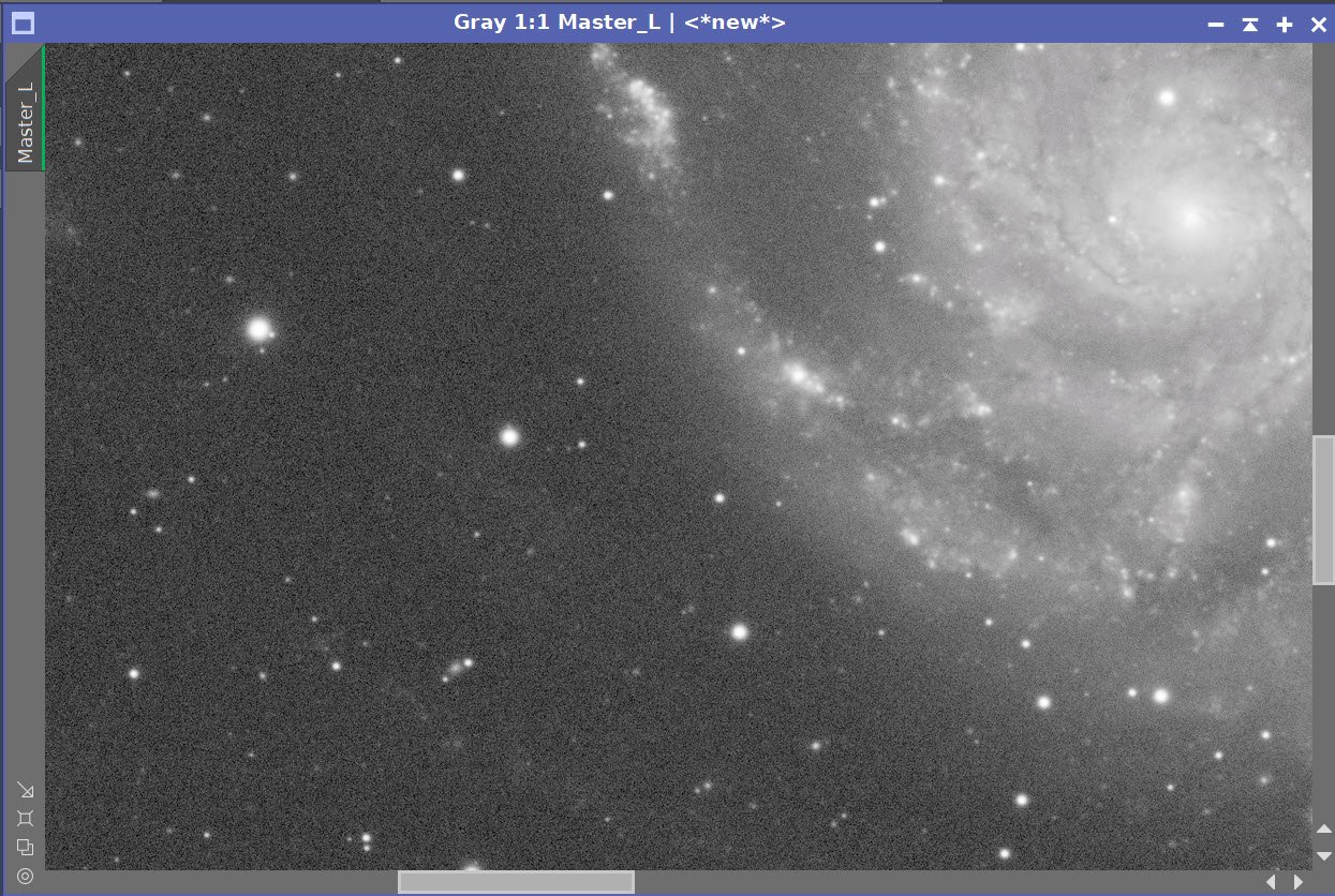
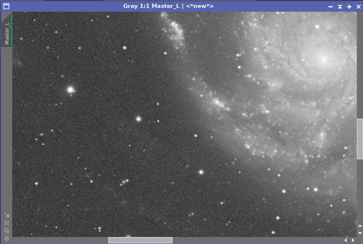
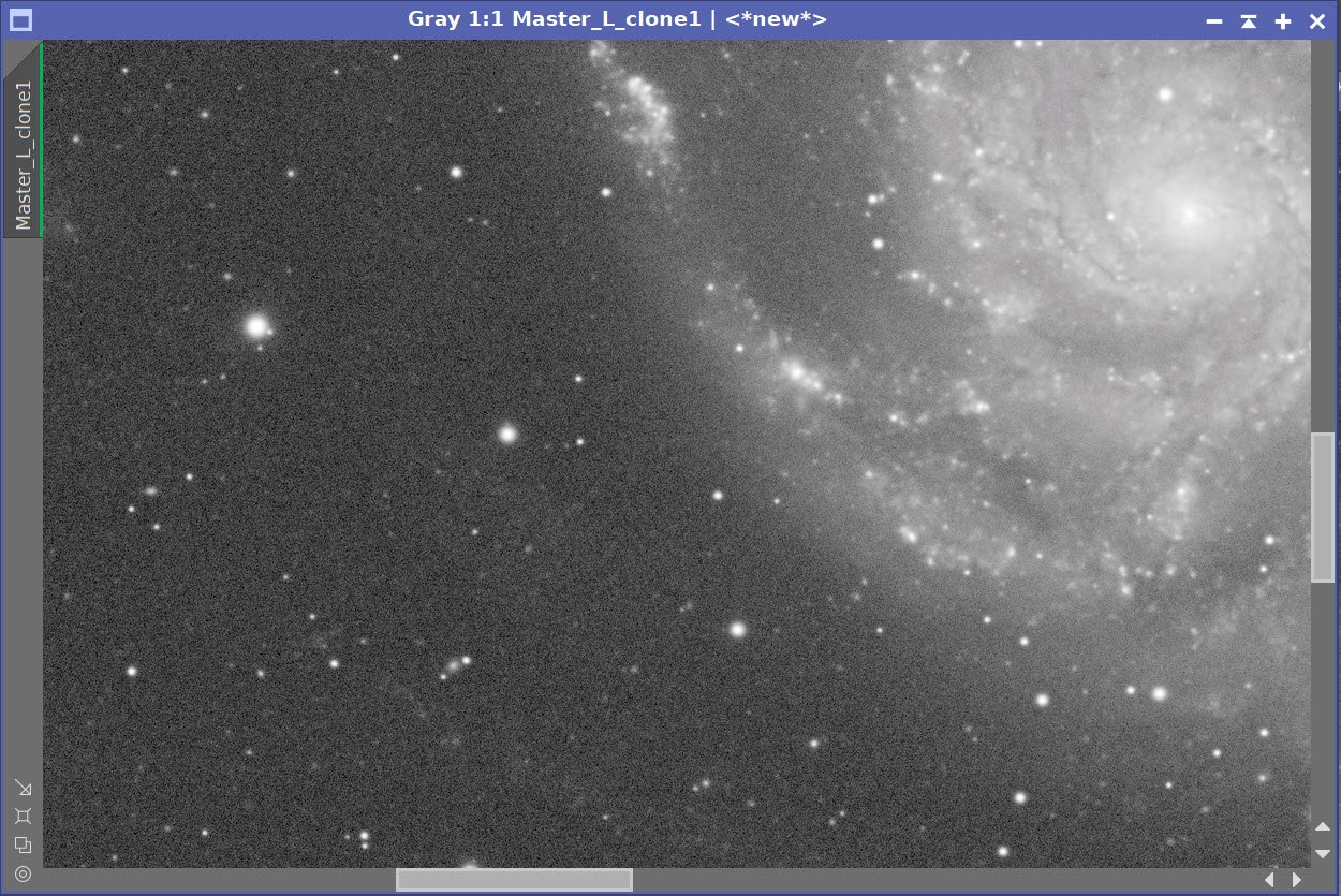
Lum Sampling (Click to enlarge)
Lum - Before DBE (click to enlarge)
Lum - After DBE (click to enlarge)
Lum - Background removed (click to enlarge)
Red Sampling (Click to enlarge)
Red - Before DBE (click to enlarge)
Red - After DBE (click to enlarge)
Red - Background removed (click to enlarge)
Green Sampling (Click to enlarge)
Blue Sampling (Click to enlarge)
Ha Sampling (Click to enlarge)
Green - Before DBE (click to enlarge)
Blue - Before DBE (click to enlarge)
Ha - Before DBE (click to enlarge)
Green - After DBE (click to enlarge)
Blue - After DBE (click to enlarge)
Ha - After DBE (click to enlarge)
Green - Background removed (click to enlarge)
Blue - Background removed (click to enlarge)
Ha - Background removed (click to enlarge)
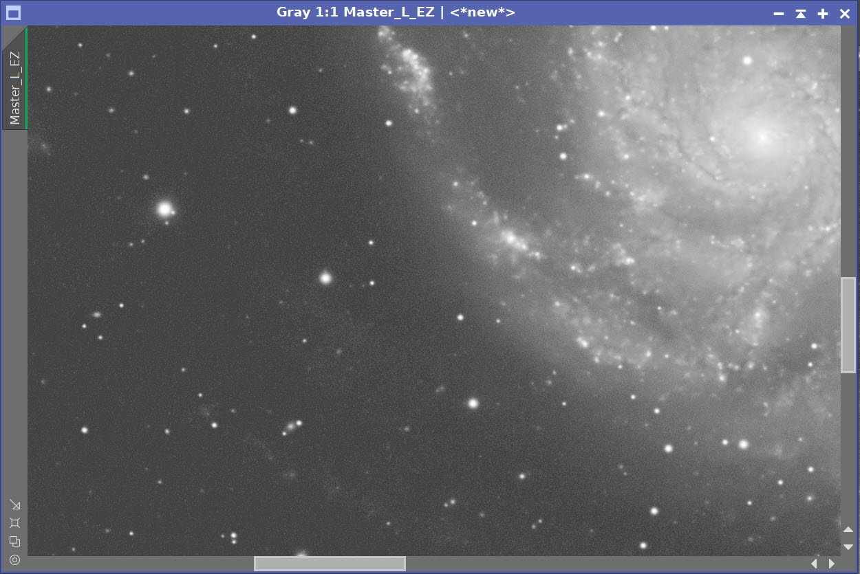
Here are the Master images - now ready for further processing.

The linear L, R, G, and B images after crop, DBE.

The Ha image after Crop, and DBE.
6.0 Linear L Processing
Prepare for deconvolution
Using the PSFImage script, calculate the PSF image for L and save it.
Create the LDSI using the Starmap Process - see Starmask Panel Below
Adjust the LDSI with HT and the morphological process to cover the star image of the larger stars in the main image

Using the PFSImage Script to create the PSF file.

The resulting PSF.

The Starmask Process setup to create the LDSI mask.
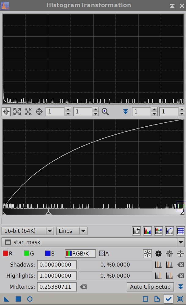
I typically use an HT curve something like this to give the LDSI maska boost before use.
Here is the final LDSI image created.
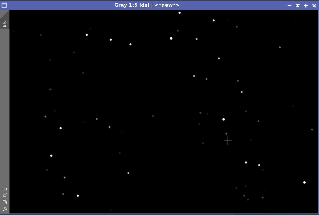
The final LDSI image.
Test parameters for deconvolution.
You might notice that I did not take the trouble to create an Object Mask for this image. That is because I no longer use them for deconvolution. With my recent article “Using Richardson-Lucy Wavelet Regularization Parameters in Pixinsight Deconvolution”, I now understand how to use the Regularization Parameters and use this to manage noise rather than use the mask method.
After doing some testing starting with the Regularization Parameter values used in my article (since that image used the same scope and camera), I finalized the values as shown below.
Apply Deconvolution
I then applied deconvolution to the whole image - see the before and after images below.

The deconvolution settings used.
Before and After Deconvolution
Do linear Noise Reduction
The goal here is to just “knock the fizz” off of the image
Typically I use MLT or EZ-Denoise at this step, but I recently bought a copy of RC Noise XTerminator and I wanted to see how that would do. So I processed the L image with it as well as EZ-Denoise. You can see the results below.
In this case, Noise XTerminator seemed a bit “blotchier” and I decided to go with EZ-Denoise.

No Noise Reduction vs. EZ-Denoise (with Defaults) vs. Noise XTerminator (0.6)
7.0 Initial Processing of the Color Image
(Note: I lost some of the screen snaps for this section, so I am missing some examples I would normally have)
Create a linear color image
Typically I create a color image by combining the RGB and then go nonlinear. The L image is then folded in with LRGBCombination in the nonlinear state. This time I decided to try a different method and see how it worked out.
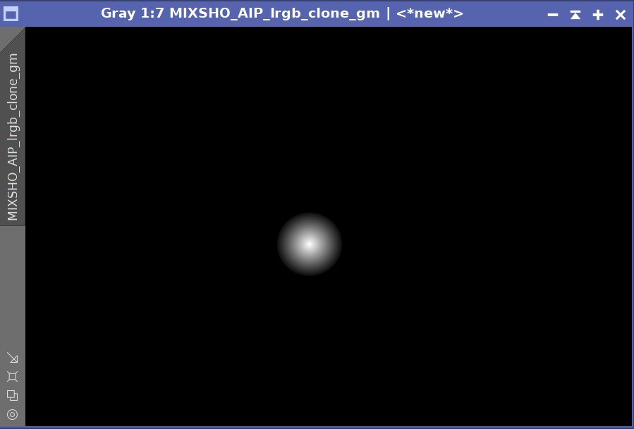
I used the SHO_AIP script to create a linear LRGB image. I added the L, R, G, & B Master Images and set the weights so the R, G, and B images were to be added at 100%. Then checked all of the boxes at the top of the panel and used the Mix L-SHONRVB button to create a mixed image. Note that I did not yet add the Ha image - that will be done later.
This created the LRGB image.
Run PCC on this image.
Used the default settings along with specific values for my scope combination
Remove Color Gradients
DBE was run on the image
Renoise the image
EZ-Denoise was run with default values.
Take the image Nonlinear
Create a Preview with an area of the background sky
Run MaskedStretch using this preview
Run CT tweak tone scale and color saturation

The SHO_AIP Script control panel with settings used.

Initial LRGB linear Image.

Final Nonlinear LRGB image
8.0 Folding in the Ha Image
Run Noise XTerminator on the Ha with a value of 0.85
Take the image nonlinear
Create a preview of an area of the background sky
Run MaskedStretch
Adjust final image with CT
Extract the Red image from the nonlinear LRGB image
Create a new combined image using PixeMath
R = (0.75Red)+(0.25*Ha)
Use PixelMath to create a new LHaRGB nonlinear image

The nonlinear Ha image, the extracted nonlinear Red image, and the 25%Ha/75%Red combine image.

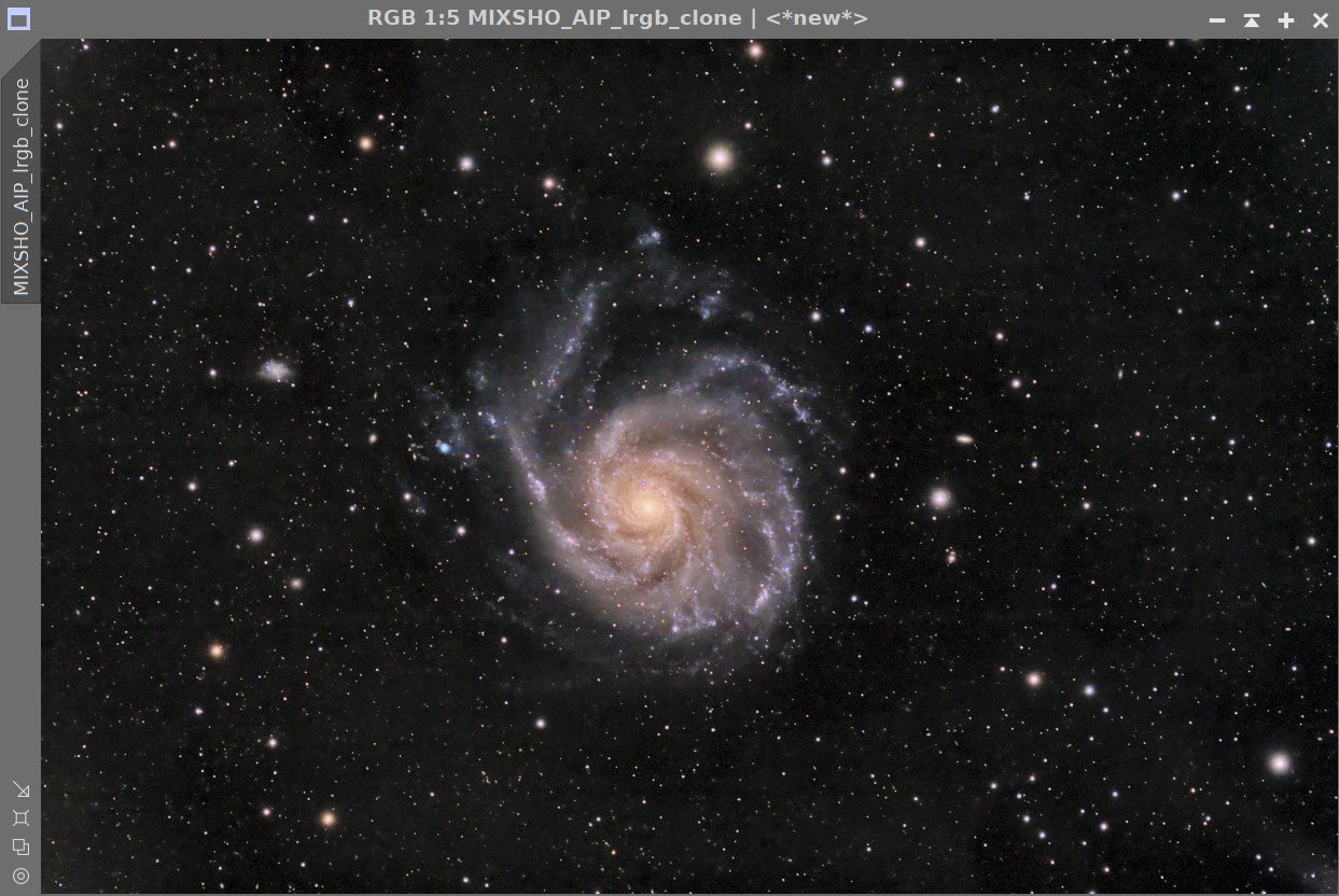
The new LHaRGB image.
9.0 Final Tweaks
Create masks for use in image tweaks:
A galaxy core mask created with GAME
A range mask created with RangeSelect to include just the galaxy
A copy of the range mask with stars removed (using DynamicPaintbrush)
Galaxy Core Mask
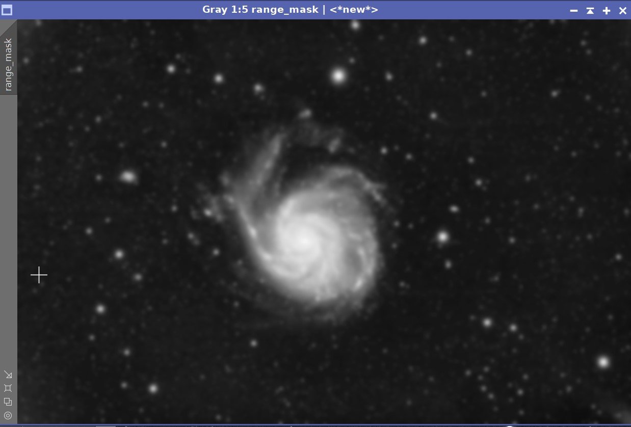
Range Mask
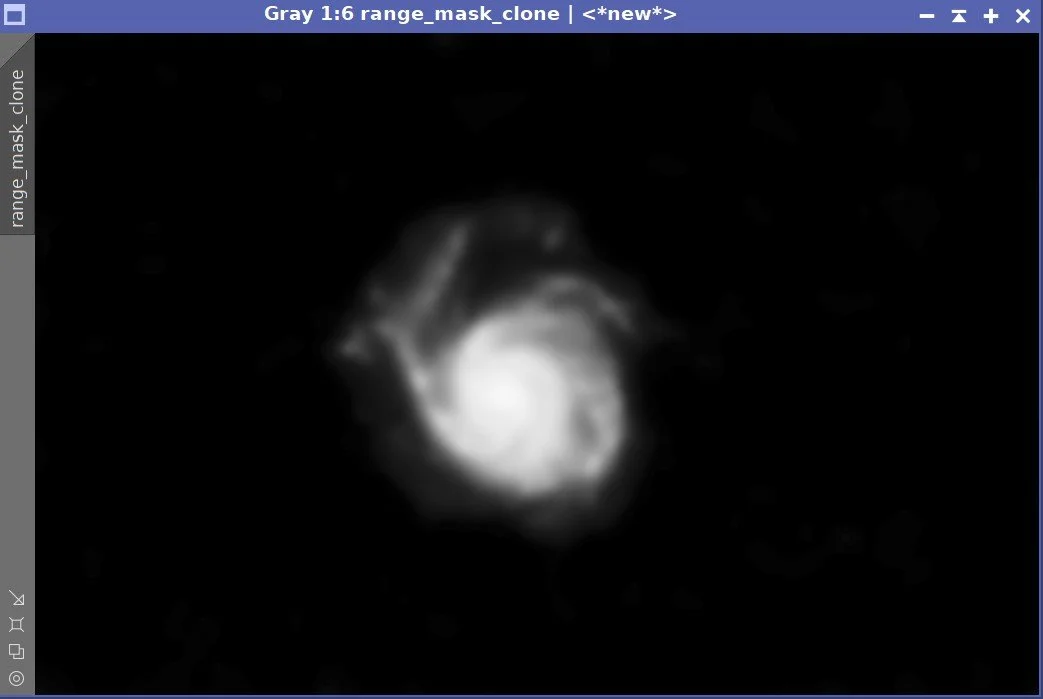
Range Mask with no stars.
Apply Core Mask
Use CT to adjust the galaxy core region making it orange-yellow warm. Exaggerate this, and make it too warm.
Use Color_Sat to Adjust the color mix in the core
Apply RangeMask with no stars
use CT to push the color of the galaxy to a blue- cool color. This will shift everything - even the core. But since we made the core too warm to begin with, it will drift into a good place colorwise with this blue shift.
Run HDRMT with 9 layers and use the Median Check box - this will daken the core region and bring out more detail
Use CT to adjust after HDRMT run
Invert the Range Mask with No Stars
Adjust the background sky color and darkness level
Use CT to adjust star saturations and color
Remove Mask

FInal color position.
Run RC Noise XTerminator with a value of 0.45. Note that XTerminator seems to do an excellent job with Nonlinear images.

Before Noise XTerminator

After Noise XTerminator
Run EZ-Star Reduction with Default values.
Before EZ-Star Reduction

After EZ-Star Reduction
10. Export to PhotoShop
Export as 16-bit tiff
Open in Photoshop
Use the Filter Starshrink to selectively reduce the bloated bright stars
Use the burn tool in shadow mode to further darken regions around bloated stars
Use Camera Raw filter to tweak color, tone, and Clarity
Carefully use Topaz AI Denoise to reduce color noise
Add in watermarks
Save image files.
Capture Hardware
Scope: Astrophysics 130mm Starfire F/8.35 APO refractor
Guide Scope: Televue 76mm Doublet
Camera: ZWO ASI1600mm-pro with ZWO Filter wheel with ZWO LRGB filter set,
and Astronomiks 6nm Narrowband filter set
Guide Camera: ZWO ASI290Mini
Focus Motor: Pegasus Astro Focus Cube 2
Camera Rotator: Pegasus Astro Falcon
Mount: Ioptron CEM60
Polar Alignment: IPolar camera
Software
Capture Software: PHD2 Guider, Sequence Generator Pro controller
Image Processing: Pixinsight, Photoshop - assisted by Coffee, extensive processing indecision and second-guessing, editor regret and much swearing….. Given the problems on this image, more than the usual whining
Adding the next generation ZWO ASI2600MM-Pro camera and ZWO EFW 7x36 II EFW to the platform…