
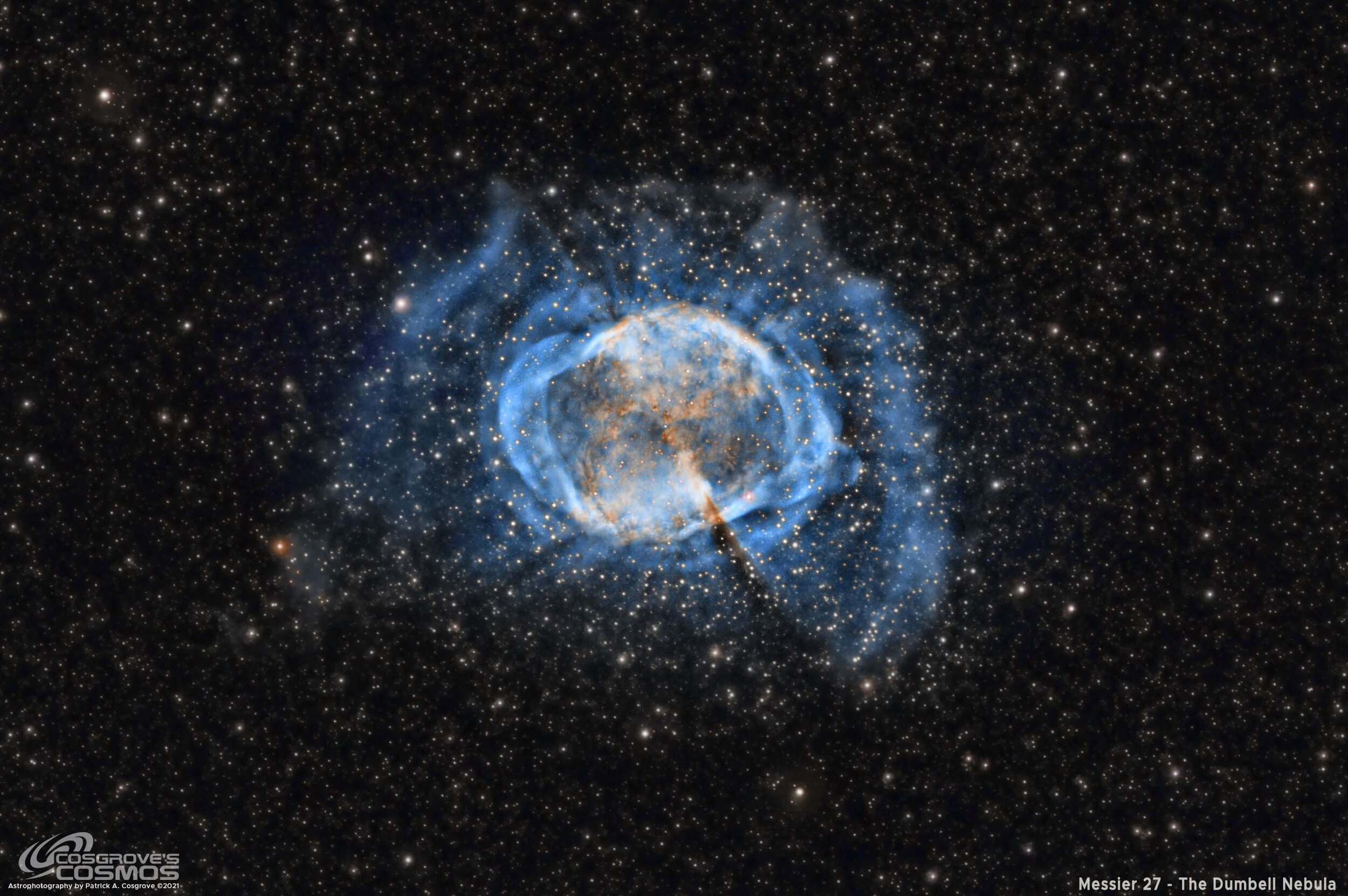
Messier 27 - A Reprocess of My Dumbbell Nebula Data in SHO - (10.25 Hours)

A preprocess of data collected a year and a half ago! (click for full res image via Atrobin.com)
Date: May 3, 2023
Cosgrove’s Cosmos Catalog ➤#0118
Awarded “Explore” Status on Flickr!

Selected As NASA’s Picture of the Day for May 30, 2023!

Published in Sky & Telescope, September 2023 Issue!


Published in BBC Sky At Night, August 2023 Issue!
Chosen as their Picture of the Month!

Grand Slam!
The original version of this image was published in Astronomy Magazine May 2022 Issue and Amateur Astrophotographer Magazine in issue #111 in April 2023.
That means that this image was selected by every publication I summited it to! This is an amazing occurrence I would not expect to see again!
Table of Contents Show (Click on lines to navigate)
Introduction
Until now, all posts in the Imaging Project area have started with the fresh capture of photons and followed how that data was collected and processed to create the final image.
This imaging project will be different.
Instead, this post will focus on reprocessing data I originally collected in September 2021. That image proved very popular and was published in Astronomy Magazine and Amateur Astrophotographer Magazine!
But I always felt a little disappointed in the final result as the stars seemed bloated and a bit blown out to me, and the details of the frill shroud around the object were not as well defined as I would like.
Now two years later, I have some new tools at my disposal and some new processing methods, so I decided to start from scratch again and see what I could do with a reprocess of that data set!
This reprocess effort has its own story, and I wanted to separate that from the previous project - so I decided to create a new imaging project post!
About the Target
For this section, I will repeat what I wrote for my original project….
Messier 27, also known as NGC 6853, the "Dumbell Nebula," and the "Apple Core Nebula," is a planetary nebula located about 1200 light-years away in the constellation of Vulpecula.
It was the first planetary nebula ever discovered by Charles Messier in 1764.
Planetary nebulae are formed when stars throw off their outer layers of gas at the end of their lives. Based on studies on its expansion rate, we can work backward to determine that the formation of this nebulae began about 10,000 years ago. Being bright and easily observable even with a small scope, M27 is famous and well-known.
The basic form of the nebula is an oblate sphere with a dimension of about eight arc minutes. There is a visual void on each side of the sphere, causing its characteristic shape. Given its size and inherent brightness, this target is easily observed and a favorite target!
Early observers debated whether this was a single nebula or two nebulae close together, and some wondered if the nebulosity consisted of unresolved stars. In John Hershel’s observing logs of 1833, he noted the following:
“h 2060 = M 27.
Sweep 166 (Auguat 17, 1828)
RA 19h 52m 8.6s, NPD 67d 43m +/- (1830.0) [Right Ascension and North Polar Distance]
(See fig 26.) A nebula shaped like a dumb-bell, with the elliptic outline completed by a feeble nebulous light. Position of the axis of symmetry through the centres of the two chief masses = (by microm.) 30.0deg .. 60.0 deg nf..sp. The diam of the elliptic light fills a space nearly equal to that between the wires (7' or 8'). Not resolvable, but I see on it 4 destinct stars 1 = 12 m at the s f edge; 2 = 12.13 m, almost diametrically opposite; 3 = 13 m in the n p quarter, and 1 = 14.15 m near the centre. Place that of the centre. “
He may have been the first person to use the descriptor of a Dumbbell - I don't know this for certain, but I can say that his observing logs were much more precise than mine ever were!
The Annotated Image

This annotated version of Messier 27 was created with Pixinsight ImageSolve and AnnotateImage scripts.
The Location in the Sky

This finder chart was created by using the Pixinsight ImageSolver and FinderChart scripts.
Video Overview
About the Project
The original data capture for this project occurred on the 1st, 4th, and 6th of September 2021. It was captured using my AP130 platform using the excellent ZWO ASI2600MM-Pro camera.
That project post can be seen HERE.
The resulting image surprised me - I was amazed by how different the Dumbell looked when shot in narrowband.
My Original Image of M27 in the SHO Hubble Palette.
This image was one that I was proud of - and the fact that it was published twice was just icing on the cake!
It was a challenge to process. The Ha, O3, and S2 images looked very different from each other, and it was not at all obvious to me how to go about processing the data. I tried a lot of options - which I wrote about in that post. It was a very challenging and satisfying project!
Some Reservations
But if I was being honest about it - I was always a little disappointed in the final result. The stars looked bloated and blown out - even a bit unsharp! And while I could show a lot of detail in the outer shell layer, I felt those areas were not as well defined as they could be. The whole image did not feel “sharp” to me.
Every time I looked at it, in the back of my mind, I thought that someday I would try my hand at processing this image once again.
Then in April of this year, I was sidelined a bit as I recovered from surgery and could not capture fresh photons.
So I used this time to work on several different projects, and when I had finished the ones I had planned, I found that I still had a bit more time. So for the past week or so - on and off - I have been playing with the data once again.
Why Would I Expect An Improvement?
I have now had an additional year and a half of experience under my belt - and I have learned a lot in that time frame.
I also had access to some advanced tools I did not have back then. Specifically:
NoiseXTerminator
BlurXTerminator
StarXTerminator
Bill Blanshan’s Star Reduction Script
These tools are powerful and, in many ways, easier to control than the methods I used to process the original Image. With those in my pocket and with some more advanced processing techniques I had learned in the interval, I felt that I could make a real improvement.
High-Level Reprocessing Strategy
Starless?
When I started this effort, I assumed I would use a starless processing method.
Since I started using StarXTerminator, my processing has used a starless approach. I even had a modified starless approach that I had been using when I folded BlurXTerminator into my processing chain.
My preferred Narrowband workflow these days looks something like this:

Preferred workflow
So that is what I set out to do. To my surprise - this approach was not working well for this image. StarXTerminator was leaving a lot of residual images behind for bright stars. This was coming through my processing, and I did not like the result. On closer inspection, there was some haze around the stars. I would guess that I had some subs with thin clouds contributing to this.
Leaving the Stars In
Given my problems with the Starless Approach, I decided to follow what I had done in the original processing and fold in some new tools and methods along the way.
So what I will do here is emphasize what I did that was different. A more complete processing walkthrough will follow below.
I planned to create a linear SHO color image early in the process and use the BlurXTerminator to enhance this color image. This takes advantage of the fact that BlurXTerminator does better star correction and sharpening when dealing with a color image, ensuring optimized processing across channels.
I found that BlurXTerminator did a wonderful job in controlling the stars, and I felt that using the traditional “leaving the stars in” method would work out well, given that.
Then I would apply the NoiseXTermintor to the linear denoise.
After this, I would break the color layers apart again and go nonlinear. This would allow me to enhance each layer image and use LocalHistorgramEqualization (LHE) to enhance small-scale and mid-scale detail in each image while using custom masks to focus my changes on various portions of the target.
Finally, I would create a Synthetic Luminance Image that was a combination of the Ha and O3 image and use this to enhance the detail of the final image. I would also process this using a two-stage LHE method to enhance the detail captured there.
Finally, I would use Bill Blanshan’s Star Reduction Script to do the final tweaks on the star.
Here is the high-level workflow I actually used:

The workflow I ended up using for this project.
Read more about this at the end of the post.
I shared the early versions of this reprocessing with my local astroimaging friends and via Twitter and Facebook. The valuable feedback I received from those communities caused me to return and take one more pass at the processing.
I backed off the star reduction and used a custom mask to reinforce the S2 data and improve the colors in the nebula's core. Finally, I softened some areas of the core that looked oversharpened.
This version of the image was chosen as my endpoint.
I've been playing around processing some old data of M27 in SHO.
— 🔭Cosgrove's Cosmos💫 (@CosgrovesCosmos) April 30, 2023
This image was processed in Astronomy Mag. I tried using some new methods.
Which do you like better?#Astrophotography pic.twitter.com/0upvQY2Pf1
This version resulting from these changes is the final one for this project.
Discussion of the Results
I hoped reprocessing this image would improve the areas I was concerned about in the original image.
I think I achieved this goal.
But is it a better image?
Many people who provided feedback on the images liked the first one better. They would say that the stars have been reduced too much and that they liked the color of the first image. Some would also say that the new image looks slightly “over-processed.”
I can see their point.
I was pushing rather hard to eliminate those aspects of the first image that I was not happy with. Perhaps I went too far.
On the other hand, most of those providing feedback thought that the new image significantly improved over the first and appreciated the added detail that can now be seen in the outer gas shells.
What do I think?
While at one level, I think I did push things a bit too far. Yet - I am still very happy with the new result. This new version is much closer to what I envisioned for this project, and I was happy to achieve this look.
Having said that, I appreciate the opinions shared with me about both versions of this image.
The nice thing about doing a separate reprocessing project is that it is not an either/or proposition. I still have the original version of the image in my collection for those that favor that rendition. But now my collection now has a new version that a lot of people may like better.
Both can coexist nicely!
Being narrowband, they are all false-color and represent some artificial presentation of the data. No one’s take is right or wrong - it’s all personal preference. And as the author of these images, I feel pretty good about the outcome!
More Information
WikipediaWikipedia: Messier 27
SEDS: Messier 27
NASA: Messier 27
Messier.objects.com: Messier 27
Capture Details
Lights Frames
Taken the nights of August 2nd, 3rd, and 4th
39 x 300 seconds, bin 1x1 @ -15C, Gain 100.0, Astronomiks 6mm Ha Filter
38 x 300 seconds, bin 1x1 @ -15C, Gain 100.0, Astronomiks 6mm OIII Filter
46 x 300 seconds, bin 1x1 @ -15C, Gain 100.0, Astronomiks 6nm SII Filter
Total of 10.25 hours
Cal Frames
30 Darks at 300 seconds, bin 1x1, -15C, gain 100
30 Dark Flats at Flat exposure times, bin 1x1, -15C, gain 100
Flats done separately for each evening to account for camera rotator variances:
12 Ha Flats
12 OIII Flats
12 SII Flats
Capture Hardware
Click below to visit the Telescope Platform Version used for this image.
Scope: Astrophysics 130mm Starfire F/8.35 APO refractor
Guide Scope: Televue 76mm Doublet
Camera: ZWO AS2600mm-pro with
ZWO 7x36 EFW
ZWO LRGB filter set,
Astrodon 5nm Ha & OIII filters
Astronomiks 6nm SII Narrowband filter
Guide Camera: ZWO ASI290Mini
Focus Motor: Pegasus Astro Focus Cube 2
Camera Rotator: Pegasus Astro Falcon
Mount: Ioptron CEM60
Polar Alignment: Polemaster camera
Software
Capture Software: PHD2 Guider, Sequence Generator Pro controller
Image Processing: Pixinsight, Photoshop - assisted by Coffee, extensive processing indecision and second-guessing, editor regret, and much swearing…..
Processing Walkthrough
This project started with the Linear Master images that came out of WBPP.
1.0 Linear Processing
All images were cropped with DynamicCrop
DBE was run on each master image to get rid of any gradients.

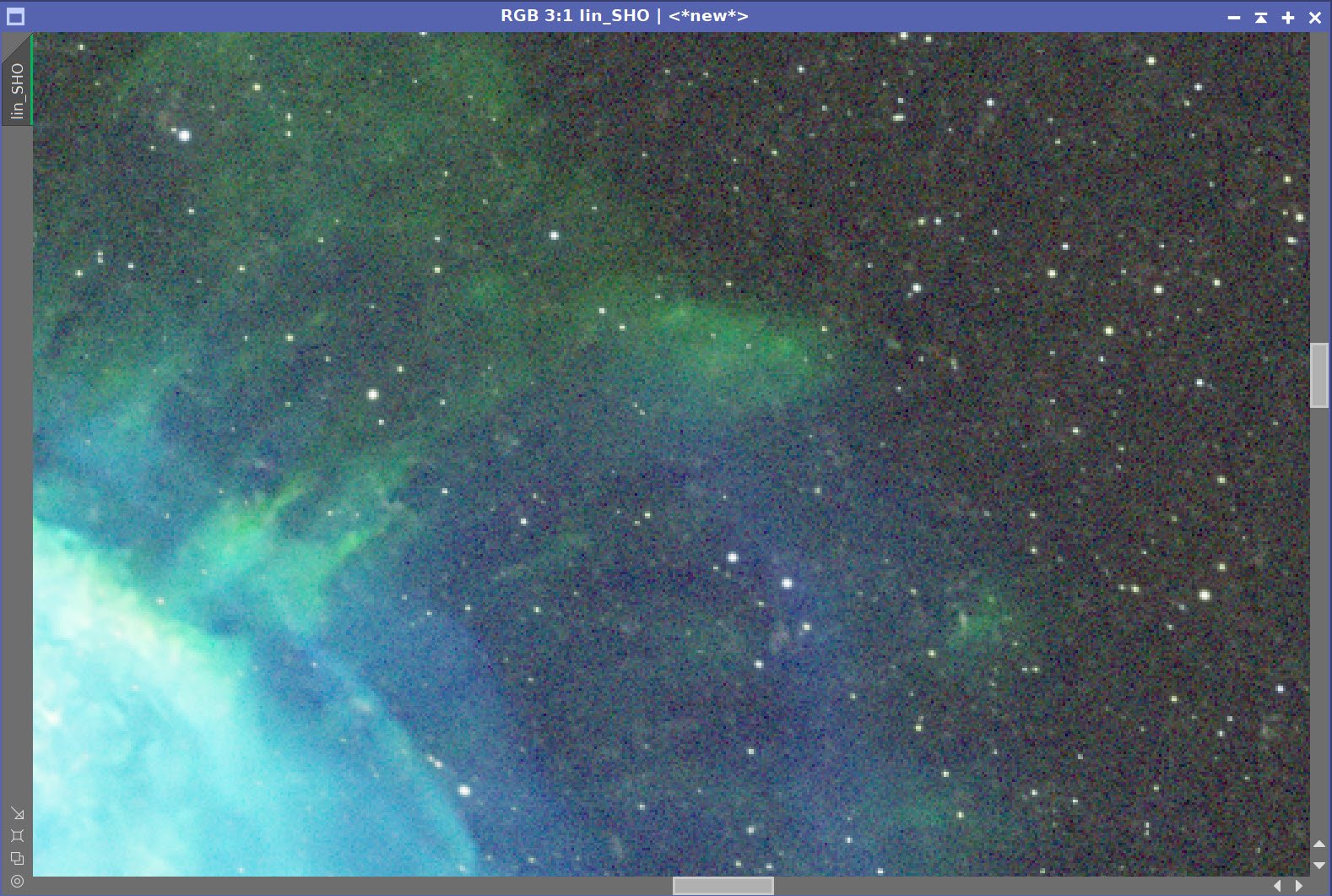
Linear Master Images: S2, Ha, O3
ChannelCombination was used to create a linear color SHO image.
Run Background normalization.
DynamicPSF tool was used to sample several stars and get the FWHM of the selected stars. This value came in at about 3.0, and I used this for BXT.

DynamicPSF was used to get FWHM star statistics that will be used for non-stellar sharpening in BXT
Run BXT:
Sharpen Stars: 0.35,
Adjust Sar Haloe: -0.18
Turn off Automatic PSF
Psf Diameter: 3.0,
Sharpen Nonstellar: 0.9
Check Correct First
I wanted to run BXT on the color SHO image, as BXT will optimize across the color layers and better deal with aberrations when in color mode. It also avoids the problem of running BXT on each color layer, and some layers have larger stars - this can cause final stars to have color rings around them. I had some of that problem with the first image.
Running “Correct First” causes BXT to circularize the stars. I do get some aberrations in the corners with AP130 scope, as I do not have a fastener. BXT helps that situation.
Showing the Impact of Just the Star Corrections with BXT
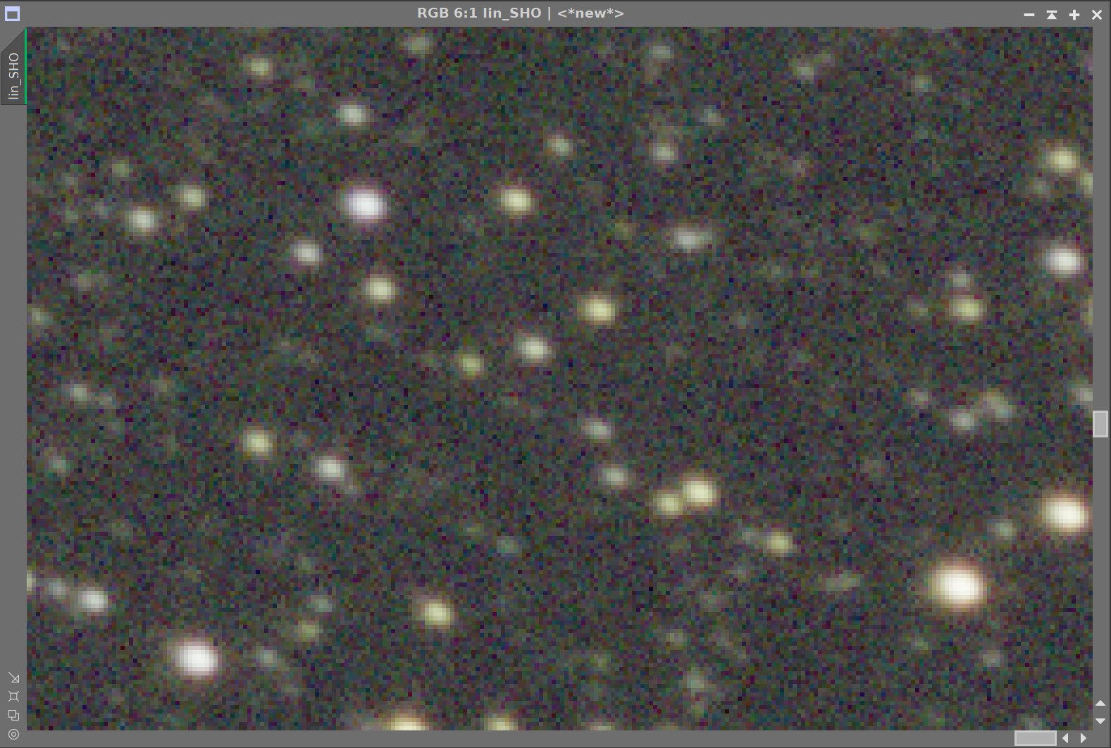
Before and After BXT Correct Only - Taken from one corner of the image.
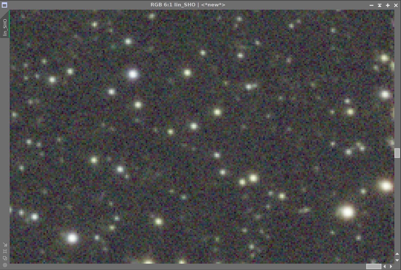
Showing the Impact of the Full BXT Process

Before and After Full BXT
This was then followed by running NoiseXTerminator - just to take the “fizz off” of the image:
Denoise: 0.55
Detail: 0.28
You can see the impact of this below:

Before and After NoseXTerminator
At this point, I wanted to return to working on each layer separately. This is because each filter layer presents such a different-looking image. You want to maximize the quality of each image separately before considering how to combine them.
Run ChannelsExtraction.
At this point, we can go nonlinear.
2.0 Nonlinear Mono Processing
For this processing session, I went nonlinear for each image by doing a masked stretch and following up with a CurvesTransformation ( CT) tweak.
2.1 Process the S2 Image:
Do MaskedStretch
Do a CT Tweak
Create a Core mask that covers the core of the target
Apply the Core Mask
Apply LocalHistogramEqualization (LHE) for finer scales
Radius=46, Slope limit=2.0, Amount 0.18, 8-bit histogram
Do a CT adjust
Invert the Core mask
Apply CT to adjust the background sky
Invert the Core mask so that the core is the focus
Run HDRMT with levels = 6
Run CT and restore lost contrast
Remove Mask
Run a Final CT
The S2 Core Mask (click to enlarge)
S2 image after Masked Stretch (click to enlarge)

S2 with core mask and running LHE and CT (click to enlarge)
S2 with the Inverse Core Mask CT adjustment (click to enlarge)
S2 image after applying the core mask and running HDRMT and CT - This is the final S2 image. (click to enlarge)
2.2 Process the Ha Image:
Do MaskedStretch
Do a CT Tweak
Create a Core mask that covers the core of the target
Create a RangeMask that covers just the shroud nebula around the core
Apply the RangeMask
Apply LocalHistogramEqualization (LHE) for finer scales
Radius=64, Slope limit=2.0, Amount 0.18, 8-bit histogram
Apply LocalHistogramEqualization (LHE) for moderate scales
Radius=210, Slope limit=2.0, Amount 0.18, 10-bit histogram
Apply the Core mask
Apply MDRMT to bring out core details with level=6
Apply CT to adjust the final contest of the core
Remove Masks
Do a final CT
Let's look at how these images have evolved.
Ha RangeMask (click to enlarge)
Ha after a MaskedStretch (click to enlarge)
Ha with RangeMask and LHE1 and LHE2 (click to enlarge)
Ha Core Mask (click to enlarge)
Ha with RangeMask and CT adjust (click to enlarge)
Ha with CoreMask and HDRMT + CT Adjust (click to enlarge)
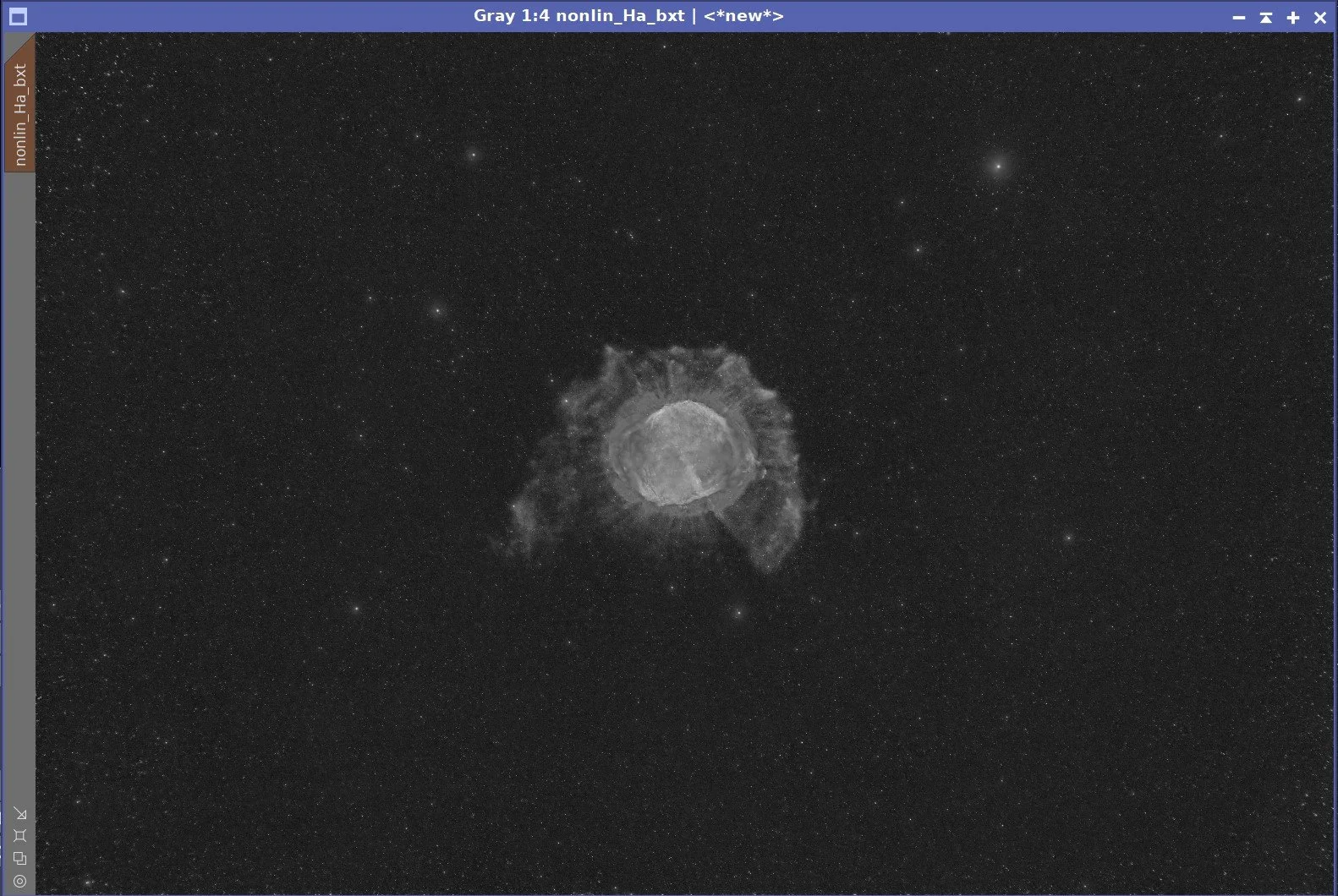
Ha with a Final CT Adjust - This is the final Ha image.
2.3 Process the O3 Image:
Do a MaskedStretch
Do a CT Tweak
Create a Core mask that covers the core of the target
Create a range mask that covers just the shroud nebula around the core
Apply the RangeMask
Apply LocalHistogramEqualization (LHE) for finer scales
Radius=56, Slope limit=2.0, Amount 0.18, 8-bit histogram
Apply LocalHistogramEqualization (LHE) for moderate scales
Radius=280 Slope limit=2.0, Amount 0.18, 10-bit histogram
Apply the Core mask
Apply MDRMT to bring out core details with level=6
Apply CT to adjust the final contest of the core
Remove Masks
Do a final CT
Let's look at how these images have evolved.
O3 RangeMask (click to enlarge)
O3 image after MaskedStretch (click to enlarge)
O3 after CT with RangeMask (click to enlarge)
O3 Core Mask (Click to Enlarge)
O3 after CT Adjust (click to enlarge)
O3 after LHE for small-scale, and LHE for mid-scale (click to enlarge)
O3 with HDRMT (click to enlarge)

O3 with final CT adjustments. This is the final O3 image.
2.4 Create A Synthetic Luminance Image
We will create a synthetic luminance image that focuses on preserving the delicate details in the outer shroud, as seen in both the Ha and O3 image. We will do a 50-50 bend of the two images to do this. Then we will process that image to show the best detail.
Using PixelMath, create a Lum image by adding the Ha and O3 image with rescaling.
Adjust the image with CT
Apply LocalHistogramEqualization (LHE) for finer scales
Radius=64, Slope limit=2.0, Amount 0.18, 8-bit histogram
Apply LocalHistogramEqualization (LHE) for moderate scales
Radius=232 Slope limit=2.0, Amount 0.18, 10-bit histogram
Run NoiseXTerminator with Denoise=0.6 and Detail = 0.28
Lum - Initial Image (click to enlarge)
Lum Image - after CT adjust (click to enlarge)
Lum Image after LHE for small-scale and LHE for Mid-Scale - slightly zoomed (click to enlarge)
Lum Image - after NoiseXTerminator -This is the Final Lum image-
3.0 Create the Nonlinear SHO Image
Use ChannelCombination to create the SHO image
Run SCNR for Green with 0.8 correction
Invert the Image
Run SCNR for Green with 0.8 correction
Invert the Image
Create an O3_Mask - the union of the O3 RangeMask and the O3 Core Mask.
Apply the O3_Mask and make a ColorSaturation adjustment tweaking the blues and orange colors.
Run NoiseXTerminator
Run LRGBCombination to fold in the Lum image
Do a global CT Adjust
Do a ColorSaturation Adjust with the O3_Mask- tweaking blues and enhancing red and oranges.
Apply O3_Mask
Apply LocalHistogramEqualization (LHE) for finer scales
Radius=64, Slope limit=2.0, Amount 0.18, 8-bit histogram
Apply LocalHistogramEqualization (LHE) for moderate scales
Radius=232 Slope limit=2.0, Amount 0.18, 10-bit histogram
Make a modest star reduction
Use Bill Blandshans Script
Create a copy of the SHO image
Run StarXTerminator to create the starless image
Run Script with method 2, with a parameter of 0.35
Run NoiseXTerminator
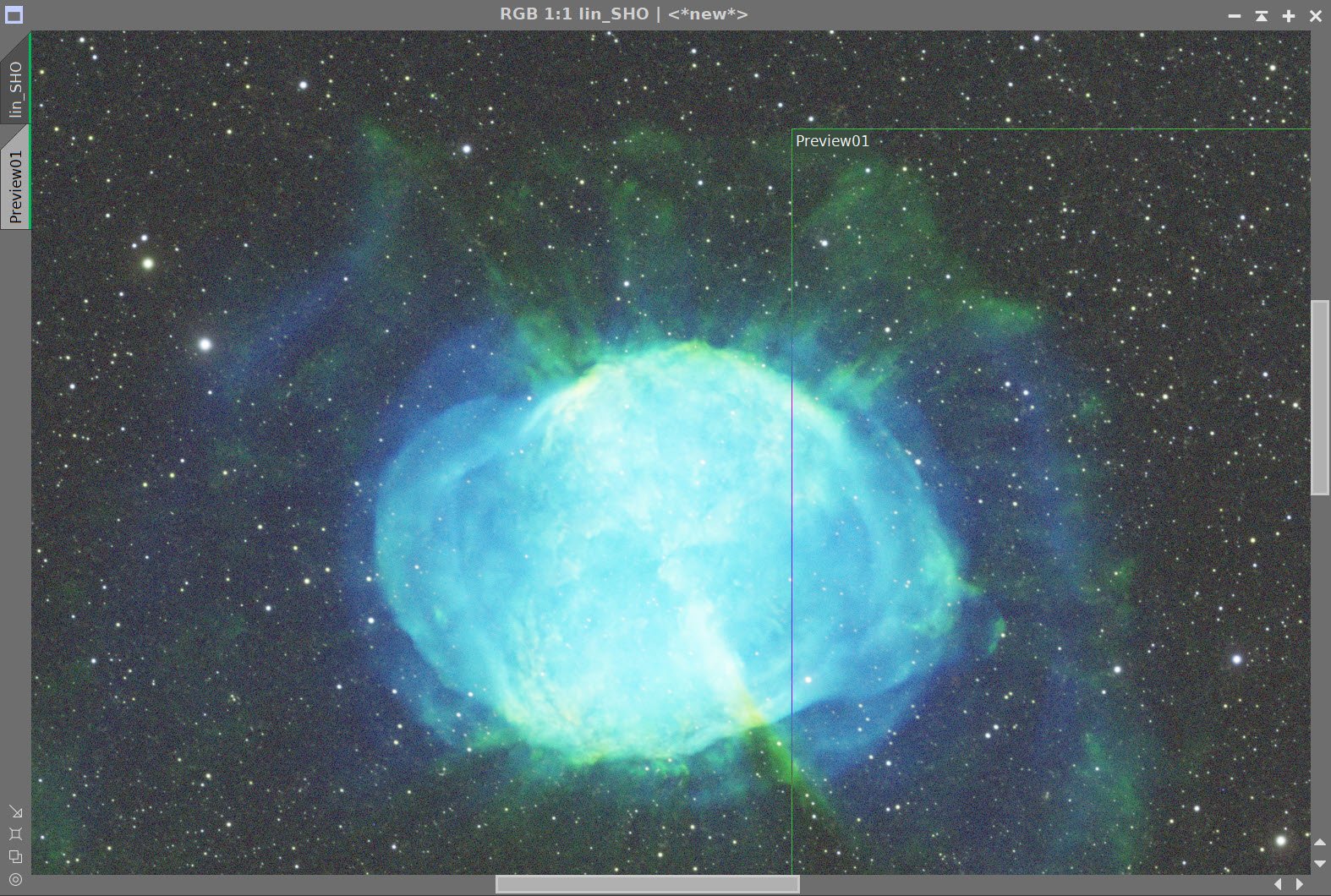
Initial Nonlinear SHO Image (click to enlarge)
SHO Image Inverted (click to enlarge)
SHO image Inverted back to correct state (click to enlarge)
SHO after Lum image Insertion (click to enlarge)
SHO with ColorSaturation adjust with O3_Mask (click to enlarge)
SHO after SCNR Green with 0.8 (click to enlarge)
Inverted SHO after SCNR Green with 0.8 correction (clikc to enlarge)
SHO after ColorSaturation Adjustment with O3_Mask (click to enlarge)
SHO after global CT adjust (click to enlarge)
SHO with LHE for small-scale and LHE for mid-scale with O3_Mask (click to enlarge)
SHI with a Star Reduction (Click to enlarge)
4.0 Export the Image to Photoshop and Do a final polish
Using Camera Raw, Tweak Clarity, Curves, and ColorMix
Crop image
Add Water Marks
Export

Initial Reprocessed Image
5.0 Initial Feedback
At this point, I was fairly happy with the image.
It had brought the stars under control and brought out a lot more detail in the shroud area. But it looked a little over-processed to me, and the orange colors were not as well defined as in the original version.
Accentuating the detail in the Ha and O3 images seems to have swamped out some of the S2 core signal.
But I wanted to get some other opinions, and I shared the original version of the image with my new version with my local Astrophoto colleagues and on Twitter and Facebook. I received a lot of really good feedback!
While a vast majority liked the new version, there were some issues that I wanted to try and address:
The star reduction might have been too much - back off a bit.
The top and bottom portions of the core region look over-processed or sharpened and don’t look natural.
I needed to get more color back from the S2 image.
6.0 A Final Pass
I returned to Pixinsight and backed off on the Star Resuction a bit.
More importantly, I created a luminance mask of the S2 image and then edited it to remove all of the star leaving just the core.
I then used this as a mask while I used the curves tool to enhance the colors from the S2 image.
The S3 image Edited Luminance Mask (click to enlarge)
SHO - where we left off before. (click to enalrge)
SHO After S2 Lum Mask applied and CT adjust (click to enlarge)
This was then exported to Photoshop, where the same polishing was done. In addition, some Gaussian blur was added to the over-sharpened portions of the core. Below is the before and after versions.

The original Image.

The initial Preprocessed Image.

The Final Reprocessed Image based on feedback.
Adding the next generation ZWO ASI2600MM-Pro camera and ZWO EFW 7x36 II EFW to the platform…